The US-China Trade War and Global Reallocations

Pablo Fajgelbaum, Pinelopi Goldberg, Patrick Kennedy, Amit Khandelwal and Daria Taglioni. This is the published version, AER: Insights 6(2), June 2024, pp. 295–312. Video used: Fajgelbaum presenting an early draft (“Trade War and Global Reallocation”) at the seventh SIDPA meeting of 2021, held on 21 October 2021, discussed by Irene Brambilla (UNLP), 98 minutes. The talk is in Spanish and the transcript is YouTube’s machine translation, so what is reported from it here is paraphrase rather than quotation, and some numbers on the 2021 slides differ from the published ones. A good deal of the paper’s apparatus sits in the online appendix rather than in the article, which carries no tables at all and only Figures 1 through 4: the Proposition 2 case taxonomy, the regression tables behind Figure 1, the micro-foundation of the supply slope, and five of the six tariff elasticities. That is flagged below wherever the argument leans on it. Figures are cropped from the published version.

Who profits from a fight between two other people

The 2018–19 trade war covered about $450 billion of trade, and the first generation of papers on it, this group’s own Return to Protectionism included, established that the tariffs were paid almost entirely by the country that imposed them and that U.S.–China bilateral trade fell in the taxed products — a confirmation this paper carries in a footnote and in online Appendix Figure A.3, with no picture of it in the article itself. That leaves the rest of the world, which the paper calls the bystanders, and which Brambilla in her discussion called the countries that were standing still when the fight hit them. The textbook prior for bystanders is trade diversion: if the United States stops buying a product from China, it buys it from Vietnam, and Vietnam sends the United States the units it would otherwise have sent to Germany. Under that prior the bystander’s exports to the rest of the world should fall when its exports to the U.S. rise, because a country’s export supply slopes up and a unit sold in one place is a unit not sold in another. The paper’s first finding is that the prior is wrong on average. In products the United States taxed, bystanders sold more to the United States (elasticity 0.31) and also more to everyone else (0.20); in products China taxed, bystanders sold nothing extra to China (0.01) but again more to the rest of the world (0.29). The war created export opportunities rather than reshuffling them.

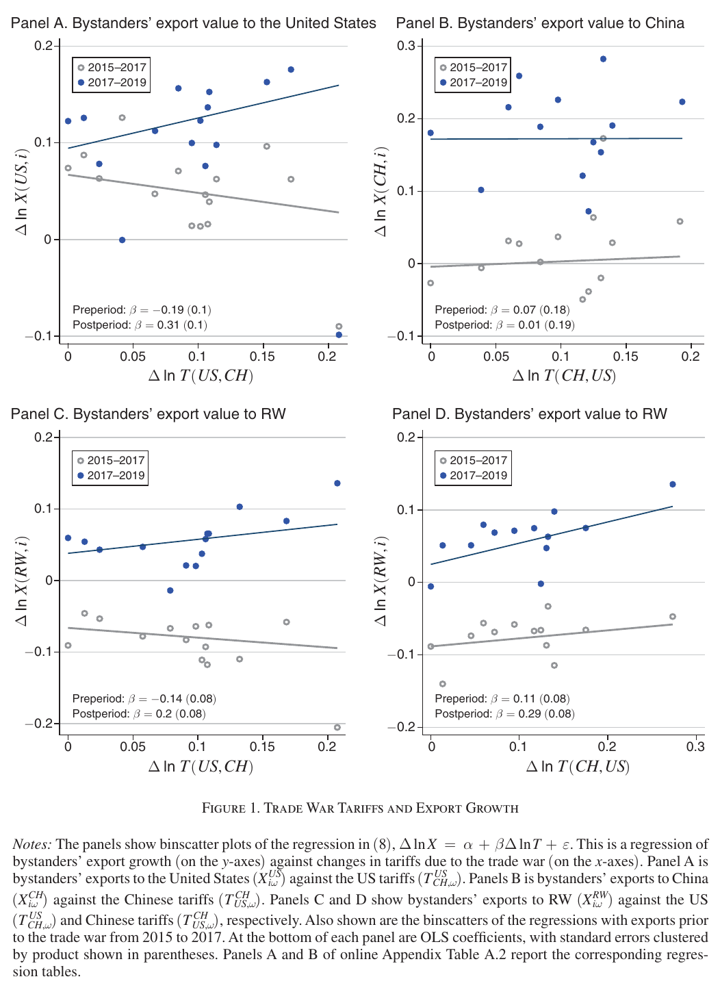
The identification is within-country, across products. Tariffs changed by different amounts on different six-digit product lines, so the regression asks whether a country’s exports of heavily taxed lines grew faster than its exports of lightly taxed lines, to each of three destinations (the U.S., China, the rest of the world), with origin-destination-sector fixed effects and the 2015–17 growth as a placebo. Three of the four grey placebo lines in Figure 1 are flat or slightly negative, which is what one wants; the fourth, panel D, already slopes up at 0.11 before the war starts, small next to the 0.29 it reaches afterwards but not nothing. Brambilla’s summary of the trade-off, which Fajgelbaum accepted, is that this buys a clean reduced form at the price of assuming that products move together, so the design cannot see interdependence across them. The published specification is less stark than she put it: equation (9) lets the elasticity vary by importer-sector across nine sectors and by the size of the trade flow, so soybeans and cars sit in different sectors with different coefficients, and the restriction that products react alike binds within a sector rather than across the whole basket.

What a tariff elasticity tells you about supply

The reason this is an AER: Insights paper and not a descriptive note is a pair of propositions that turn those elasticities into statements about structure. The model is Ricardian-Armington with two liberties. On the demand side, substitution is country-pair specific: Mexican goods can substitute for Chinese goods in the U.S. market while complementing American ones, and for another exporter the signs can be reversed. On the supply side, each country-sector has an inverse supply elasticity $b_i^j$ that may be negative. A first-order expansion of the equilibrium gives the elasticity of exports of product $\omega$ from bystander $i$ to a destination $n$ with respect to the U.S. tariff on China (equation 6, p. 300):

where $\sigma^j_{CHi}$ is the cross-substitutability between Chinese and $i$’s varieties, $\sigma^j_{ii}$ the own semi-elasticity, and the size ratios are pre-war shares. The structure is worth reading slowly, because it is the whole argument: the ratio $\sigma^j_{CHi}/s^n_{i\omega}$ multiplies everything, so the sign of the elasticity is carried by the cross-substitutability alone, while inside the bracket the indicator is the direct demand hit that only the U.S. market feels and the second term is the general-equilibrium price adjustment, whose magnitude and sign turn on $b^j_i\sigma^j_{ii}$ measured against the exporter’s world market share. The counterpart elasticities for the Chinese tariffs and for the four other tariff terms are not in the article at all; they are equations (B.31) through (B.35) of the online appendix. Proposition 2 is the useful part. If the U.S. taxes China, then whether $i$’s exports to the U.S. rise or fall reveals the sign of $\sigma_{CH,i}$ (substitute or complement), and given that, whether $i$’s exports to the rest of the world move in the same direction as its exports to the U.S. reveals the sign of $b_i$. Neither step is unconditional: the first holds only over a range of $b^j_i\sigma^j_{ii}$ relative to the exporter’s world market share, which the paper’s footnote 10 argues is guaranteed once the number of countries grows large or when the United States does not command a very large share of the world market, and the second requires own demand to slope down. Same sign in both destinations means downward-sloping supply: extra demand from one buyer made the country cheaper for every buyer. Opposite signs mean the familiar upward slope and diversion. The full case table is online Appendix Table A.1; the article only points at it. The tempting move is to feed the average finding above — up in the U.S., up in the rest of the world — through this lens and call the average bystander a substitute for China on a downward-sloping supply curve, and the paper explicitly blocks that reading on p. 304: the average country is revealed to neither complement nor substitute China, and a null average can perfectly well hide countries substituting and countries complementing in equal measure. The taxonomy belongs on the country-level estimates, which is where the paper puts it.

The heterogeneity is in the country, not the product mix

The paper then lets the elasticities vary by exporter, by sector and by the size of the trade flow, and aggregates product-level predictions with pre-war export weights to get each country’s predicted growth in taxed relative to untaxed products. The mean is 6.4 percent with a standard deviation across countries just as large, 6.2 percent. Thailand gains 14.6 percent and Mexico 9.1; Ukraine loses 11.3 and Canada gains 1.2.

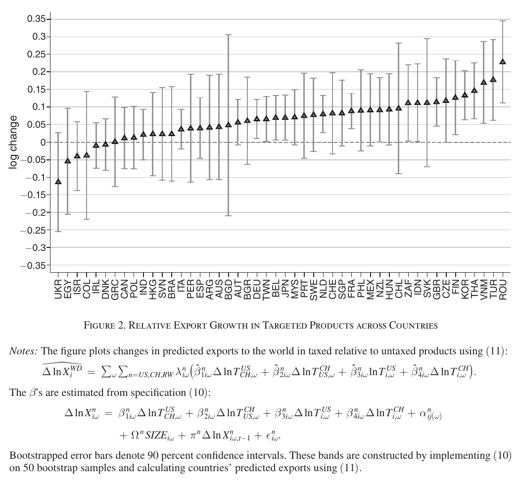
One would expect that dispersion to come from specialization: Vietnam happens to make the things the U.S. taxed, Canada does not. It doesn’t. Shutting down all elasticity heterogeneity and keeping only specialization produces a standard deviation of 1.4 percent and essentially no cross-country variation. Sector-specific elasticities get to 4.0 percent with a correlation of 0.37 with the full estimate; size-specific elasticities explain nothing; the country-specific component alone gets to 6.0 percent with a correlation of 0.78. A formal decomposition puts 75.8 percent of the cross-country variance on the country component. This is the finding the authors flag as surprising, since trade and scale elasticities are conventionally allowed to vary by sector and assumed common across countries; here the sector is nearly irrelevant and the passport is everything. Those six numbers all come off Figure 3, which is the nearest thing the article has to a table.

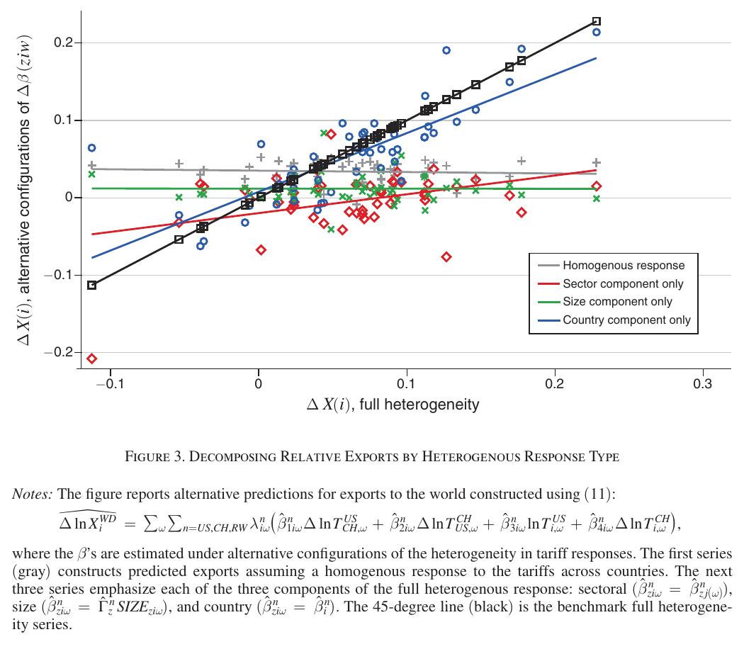
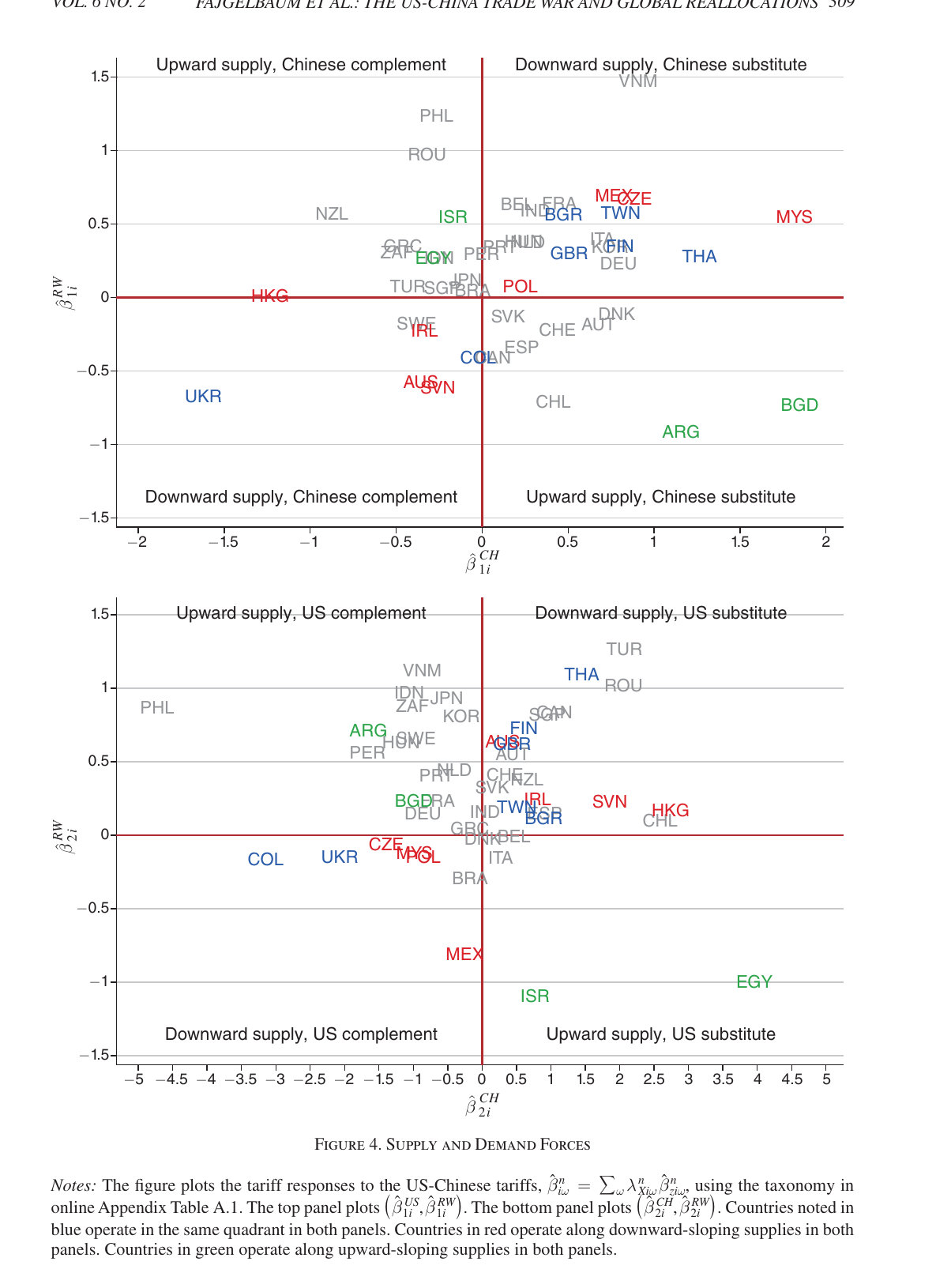
Figure 4 is the taxonomy applied, its quadrant labels tracking a case table that is itself in the online appendix rather than the article. Thailand, Taiwan, Britain, Bulgaria and Finland sit in the northeast quadrant of both panels: substitutes for both combatants, downward-sloping supply, the clear winners. Ukraine and Colombia sit in the southwest of both: complements to both combatants on downward-sloping supply, so the tariff cut their sales to the U.S. and China and the lost scale then cut their sales to everyone else. Mexico, Malaysia and the Czech Republic substitute for China in the U.S. market but complement the U.S. in China’s, and operate on downward-sloping supply in both. The grey countries flip between panels, which the model cannot accommodate without a further source of heterogeneity; the authors point at bilateral supply elasticities (Lind and Ramondo) or destination-specific trade-cost complementarities (Alfaro-Ureña et al.).

What the room pushed on

Brambilla’s main objection was to the language of “downward-sloping aggregate supply.” Her point was that the phenomenon is really positive interdependence across destinations, which can come from value chains, from fixed costs, or from firms, and she cited her own work with Albornoz and Ornelas on the 1997 U.S. suspension of Argentine tariff preferences, where firms that stopped exporting to the U.S. also stopped exporting elsewhere — a scale or fixed-cost effect at the firm level that the product-level regression cannot see — while at the product level within a firm the sign was the opposite, substitution. Fajgelbaum’s reply was that the model in the paper is there to state the assumptions that make the regression coherent, that its micro-foundation already splits $b_i$ into a factor-mobility term and a returns-to-scale term, and that an earlier draft had the country component on the first and the sector component on the second before they simplified it; he said they should revisit that. The question that drew the longest answer was from the floor: why not estimate product by product? His answer was that the only variation is across products, so a product-by-product estimate has nothing to identify off, and that the choice to privilege country-pair heterogeneity in substitution over product heterogeneity was deliberate. He also offered the interpretation the published paper keeps at arm’s length: China responded to U.S. tariffs by exporting more to third markets, so the rest of the world was gaining share there against a cheaper Chinese competitor, which to him is what makes the scale story more plausible than a pure demand story.

Where it sits

The paper’s conclusion is unusually blunt for a 2024 trade paper: the trade war, over the horizon they study, was not the turning point in globalization it is routinely described as, because several countries grew their global exports in exactly the products the two giants taxed. For the fragmentation literature it is the product-level, causal counterpart to the gravity evidence in Gopinath et al.: where that paper shows connector countries appearing in the aggregates, this one shows the mechanism by which a connector becomes one, and that it is a country-level property rather than a product-mix accident. It also quietly raises the stakes for the “de-risking” debate, since a bystander on a downward-sloping supply curve is a bystander whose dependence on Chinese inputs may have risen with its U.S. market share, which is the conundrum Gopinath et al. state and Alfaro and Chor measure.