Trade Fragmentation, Inflationary Pressures and Monetary Policy

Ludovica Ambrosino (LBS), Jenny Chan (Bank of England), Silvana Tenreyro (LSE). Journal of International Economics 163 (2026) 104219, 23 pages, in the “ISOM 2025” special issue; open access under CC BY, with replication files on Mendeley Data. Page references below are to the published article, which supersedes the January 2026 preprint; the appendices are now online supplementary material and carry no article figure numbers. Video: Chan presenting at the ECB’s “Inflation: Drivers and Dynamics” conference, 29 September 2025 (session chaired by Elena Bobeica), discussed by Giancarlo Corsetti; 48 minutes including Q&A. Tenreyro also gave the paper as a 60-minute CEPR Virtual Seminar on Monetary Economics in December 2025, not used here. Figures are cropped from the published article; the slide is a frame from Corsetti’s discussion.

The conventional view, and what it leaves out

Central bankers have said, more or less in chorus, that fragmentation will be inflationary: supply chains duplicate, firms buy from friendly rather than cheap suppliers, costs rise, and the disinflation of the 1990s and 2000s that was credited to globalization runs in reverse. The paper’s complaint about this view is that it is partial equilibrium. Higher import prices raise marginal cost, yes. They also make the country poorer, and a poorer country spends less, and a country that spends less has lower domestic inflation, a lower natural rate of interest, and — depending on the balance — may need monetary policy to loosen rather than tighten. Corsetti’s first slide put the theoretical point in one line: there are no supply shocks and demand shocks, there are shocks with supply and demand effects, and with incomplete markets the wealth effects on demand can be large.

So the answer to “is fragmentation inflationary?” is that it depends on how demand adjusts, and the paper’s contribution is to say precisely on what. Chan’s opening at the ECB gave the short version: will fragmentation lead to a high-inflation environment? In principle no — with an inflation-targeting central bank, inflation returns to target. Will it generate inflationary pressures along the way? It depends, above all on whether fragmentation arrives gradually or all at once.

The model

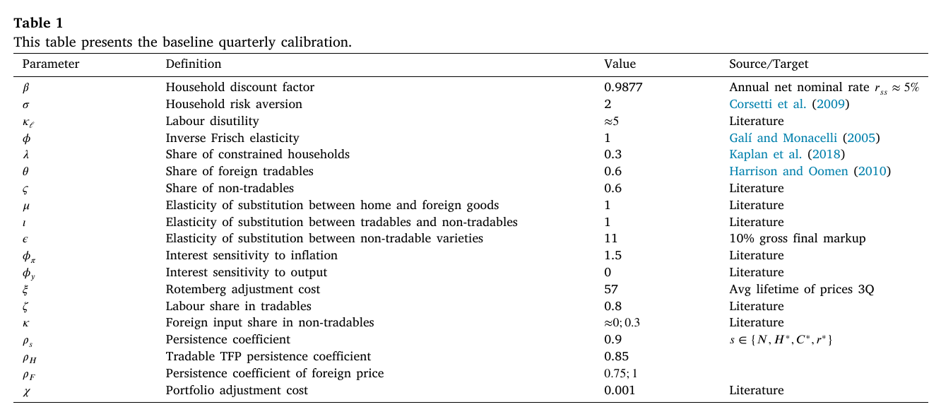
A two-sector small open economy in the Galí–Monacelli tradition: a non-tradable sector with sticky prices (Rotemberg) and a flexible-price home tradable sector, home bias in consumption, and imports used both for consumption and as an intermediate input in production. Two kinds of household, following Debortoli and Galí: unconstrained households that trade domestic and foreign bonds — with a convex cost of deviating from a long-run foreign-asset position (Schmitt-Grohé–Uribe), so international risk-sharing is imperfect and UIP fails — and hand-to-mouth households who consume their wage. The share of the latter, $\lambda$, is 0 in the RANK benchmark and 0.3 in the TANK baseline. Fragmentation is either a permanent rise in the foreign price level (tariffs, non-tariff barriers, switching to dearer aligned suppliers) or a permanent fall in home-tradable TFP (losing the productivity gains that trade integration brought). Monetary policy follows a Taylor rule, and the decentralized outcome is benchmarked against a constrained-efficient allocation in the manner of Drechsel, McLeay, Tenreyro and Turri.

One line of the calibration deserves to be read out loud, because of what it switches off. The parameter $\kappa$ — the share of the imported input in non-tradable production, the thing that carries higher import prices straight into the marginal cost of the only sticky-price sector in the model — is set close to zero in the baseline. The headline disinflation result therefore does not travel through imported intermediates at all. There is no cost-push through the supply chain in the figure everyone will quote; there is only real income and anticipation, working through the consumption basket. The authors are open about it and show that a positive $\kappa$, around 0.3 to match the non-labour share of income, amplifies the fragmentation scenarios while leaving the qualitative reading unchanged, which is a fair defence. It is still the kind of thing a reader should know: the paper’s most contrarian result is obtained with the most conventional-sounding channel turned off, and it does not need that channel to get there.

Three scenarios

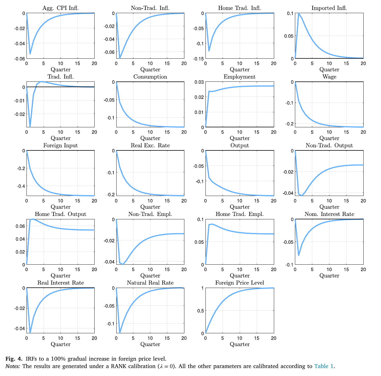
The gradual, permanent import-price increase is the case that overturns the conventional view. Imported inflation rises and stays positive for years as the foreign price climbs. But consumption falls from the first quarter, because unconstrained households see the permanent-income loss coming and cut spending now; real wages fall from the terms-of-trade loss and from weaker demand; non-tradable inflation and home-tradable inflation both turn negative; and because domestic goods dominate the basket, aggregate CPI inflation falls. The natural real rate drops. The central bank following its Taylor rule cuts. The economy settles into a long stagnation — lower consumption, output and wages, higher employment as households work more to offset lost income — with inflation below target throughout. Fragmentation that arrives slowly is a demand shock wearing supply-shock clothes.

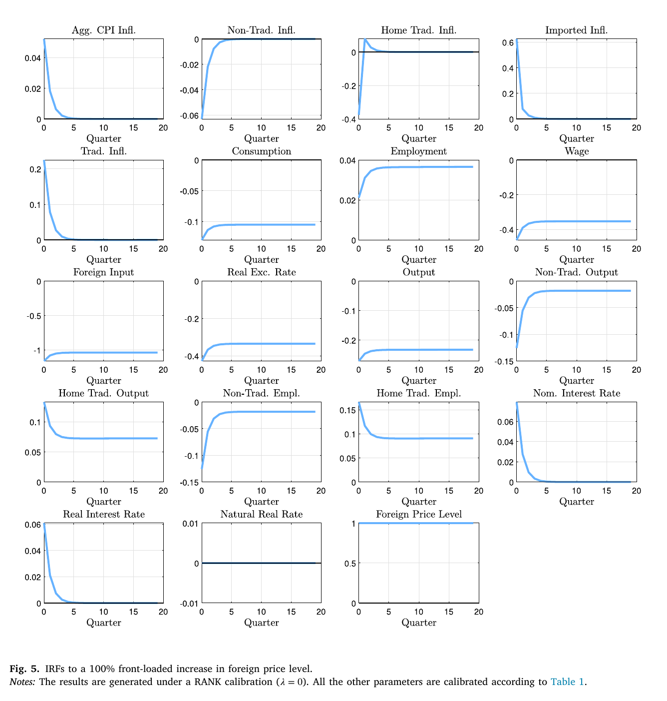
The front-loaded permanent increase is the stagflation case (Fig. 5, p. 12). Import prices jump at once; inflation rises on impact while demand falls; the central bank faces a genuine trade-off, raises the real rate, and buys a temporary inflation overshoot with a longer-run loss of income. The natural real rate, though, does not move at all: its panel is a flat line at zero. The trade-off is not that the neutral rate has shifted under the bank’s feet, as it does in the gradual case; it is that the bank deliberately opens a positive real-rate gap against an unchanged natural rate, and pays for the inflation it buys back in lost income. The paper’s footnote offers the 2024 EV tariffs and the post-invasion energy shock as examples. Corsetti’s reading was that this is the case one would motivate with low short-run substitution elasticities — a geopolitical disruption that targets a critical input — and Chan agreed that if the shock is meant to be geopolitical, low short-run and higher long-run elasticities are the right way to think about it.

The gradual TFP decline in tradables — a permanent fall of 10 percent (Fig. 6, p. 13) — sits between. Marginal costs rise in home tradables, employment per unit of output rises, real wages fall less than in the price-shock case, so consumption falls less; the fall in non-tradable inflation does not fully offset the rise in home-tradable inflation and CPI inflation rises moderately, with the natural rate ambiguous in principle and slightly negative in the calibration.

Heterogeneity and the planner

Adding hand-to-mouth households does two things in opposite directions. Constrained households do not anticipate, so the forward-looking cut in demand is weaker; but they are hit directly by higher prices, and the spillover from unconstrained households’ lower spending lands on them, so consumption falls more in TANK than RANK. Output falls less, because constrained households raise labour supply more. The qualitative conclusions survive: in the gradual scenario demand still falls enough to offset imported inflation. Corsetti’s comment, in his own discussion, was that in the aggregate pictures the TANK and RANK lines are almost on top of each other, and that the heterogeneity would matter more if the model let elasticities be low in the short run and high in the long run, citing the GVC-disruption literature and old work with an elasticity of 0.1.

The planner comparison isolates two inefficiencies: sticky non-tradable prices and the friction on foreign-bond adjustment. Together they produce too much reallocation toward home tradables after the import-price shocks and too little toward non-tradables after the TFP shock.

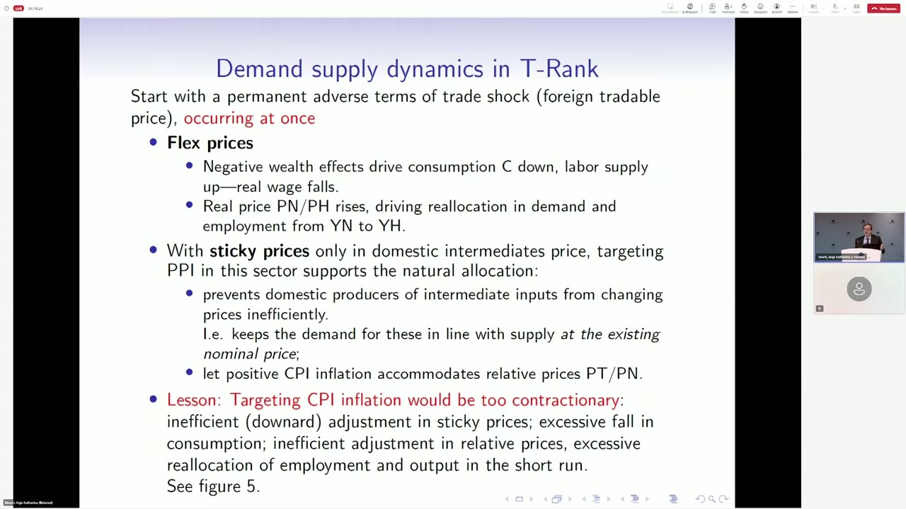Corsetti’s discussion at 00:32:55: with stickiness only in the non-tradable sector, targeting that sector’s inflation supports the efficient allocation; “Targeting CPI inflation would be too contractionary.”

What the discussant wanted

Corsetti liked the paper and spent his time on policy implications it leaves implicit. With one sticky-price sector the efficient response is to stabilize that sector’s prices and let CPI absorb the relative-price movement; CPI targeting leans against an efficient adjustment, contracts consumption too much, and forces an over-reallocation of employment into tradables that the model treats as costless and reality does not. In the gradual case, a central bank that fails to ease enough lets sticky-price firms cut prices wastefully and then has to run loose policy later to get back to target. He asked for the relative price $P_N/P_H$ to be plotted, and closed with two directions: the two-way feedback between sectoral dynamics and the income distribution, and market structure — trade disruption in oligopolistic markets with entry and exit, which Calvo-style models ignore. Chan accepted the CPI point (the paper’s planner exercise makes it, and PPI targeting gets closer but is not ideal since the home tradable sector is flexible), and emphasized that the shock is a relative-price shock with real effects, not a price-level shock. A question from the floor (apparently Guido Ascari, per the captions) argued provocatively that fragmentation is good for monetary policy because it raises the domestic share of marginal cost and so restores the central bank’s grip on inflation; Chan took the point without disputing it.

Where it sits

This is not geoeconomics in the CMS sense — there is no strategic agent, no threat, no participation constraint; geopolitics enters as an exogenous shock process. It is the transmission branch: what a small open economy’s central bank should expect when the fragmentation described in block 1 reaches it. It is on the list because the group’s own work sits here, and because it is the most complete statement of the demand-side correction to the “fragmentation is inflationary” consensus. The obvious extensions are the ones Corsetti listed plus one he did not: the shock here is trade loss (dearer imports, lower productivity), whereas the block-1 evidence says what actually arrives in a connector economy is trade rerouting, with different real-income consequences for different households. That is the gap between this paper and the empirical block, and it is where the reading group’s own contribution could go.