Friends in Higher Places: Social Fit and University Choice

Nagisa Tadjfar and Kartik Vira
Presented by Nagisa Tadjfar at the nber Economics of Talent Conference, Cambridge ma, 2 October 2026 (video). No discussant.
Paper version: the September 26, 2026 draft. Where the talk and the paper give different numbers, the text says which one it is quoting. The paper is Vira’s job-market paper.

A system built to remove every excuse

The uk has removed most of the reasons an American economist would give for why a bright poor student doesn’t apply to an elite university. Tuition is uniform (within England, for English students), loans are income-contingent and collected with your taxes, every application goes through one portal (ucas), admissions are largely test-based, and elite universities make income-based contextual offers that tell disadvantaged students outright they can get in with lower grades. And still, in the top decile of gcse scores, low-income students are up to 12 percentage points less likely to enrol at one of the ten most selective universities, and up to 12 points less likely to apply (paper p. 9). Equalising application rates would close 40–50% of the enrolment gap for the highest-ability students (p. 10).

The other fact is about whom you have seen go. Low-income students are 5–10 percentage points more likely to be at a school that sent nobody to a top-10 university in the previous three years (pp. 1–2). That students follow siblings and schoolmates is well established; what they are responding to is not. Tadjfar laid out three possibilities (00:09:50): you want to be where your friends are, which needs no information friction; you learn something general, like the application process, the grades or the earnings; or you learn something specific to a group and a university, “whether someone like them would fit in at a particular university” (00:10:31). The first says send students in batches, the second says publish a better brochure, and the third says the brochure was never the problem. The paper’s answer is the third, reached in two steps: administrative data on “breakthroughs”, and a field experiment that tries to manufacture one.

Why non-attendance persists (the model the talk skipped)

; not shown in the talk and not the authors’ exhibit. Panel (a) is the two-regime chain in which each cohort sees only the cohort before it; panel (b) shows the attendance cutoff in each regime, with the post-breakthrough cutoff falling in the predecessor’s payoff and lying below the non-attendance cutoff for any payoff above a threshold that is itself negative. Illustrative and uncalibrated: no axis values, and slopes and gaps are not to scale.’)

Section IV of the paper has a small social-learning model, never shown in the talk, of why a school stays stuck and how one student unsticks it. Your payoff from the elite university is a known common return plus a community match $\gamma$ (how students like you fare there) plus your own draw $e_t$, which you see before choosing. With cara preferences you attend if $e_t \ge \kappa_t \equiv \tau - \mu_t + \tfrac{\lambda}{2}\sigma_t^2$ (eq. 2), so the bar rises with pessimism about $\gamma$ and also with mere uncertainty about it. All you observe is last year’s student: her payoff $x = \gamma + e_{t-1}$ if she went, only her absence if she didn’t.

The load-bearing assumption is how you read that absence. You treat her as if she knew her own match and stayed away because it was low, when in fact she was looking at the same empty record you are. A rational observer would learn nothing from it, as footnote 11 says. The naive, Eyster–Rabin (2005) observer reads it as bad news about $\gamma$, and the cutoff rises above its level under the prior (Proposition 1). One student’s idiosyncratic reason not to go becomes the next cohort’s evidence about the community.

The way out is a student whose $e_t$ clears the raised bar anyway: the breakthrough student. The next cohort sees a real payoff, re-anchors its mean at $rx$ ($r$ is the community component’s share of payoff variance) and gets a larger variance cut than a non-attendance ever delivers. By Proposition 2, attendance then becomes more likely than in the non-attendance regime for any outcome above a threshold $\bar x$, and $\bar x$ is negative: a mildly bad experience still lowers the bar, because the variance cut does the work on its own. Neither regime is absorbing, and a year with nobody sends the school back (fn. 14).

The model is illustrative and uncalibrated, it is not in the abstract, and the paper uses it for the persistence story, the reading of baseline pessimism (p. 22) and the low-ses prediction (p. 24). It also undercuts one of the authors’ own arguments, which comes up at the end.

Breakthroughs

A breakthrough is the first time a school sends a student to a given top-10 university after sending none there in 2007–2009. It happens some year in 2010–2021, and schools that never break through are controls (p. 13). The data link school records to ucas applications, hesa enrolment and graduation, and hmrc earnings. The per-university event study is (eq. 5, p. 13)

where $Y_{ist}$ is an outcome for student $i$ at school $s$ in cohort $t$, $\alpha_s$ and $\gamma_t$ are school and year effects (this $\gamma_t$ is not the model’s community match), $X_{ist}$ are controls, $D_s$ marks a breakthrough school, $T_s$ is its breakthrough year and $\beta_\tau$ is the effect $\tau$ years out. The breakthrough student herself is dropped, and the paper uses the Sun–Abraham (2021) estimator.

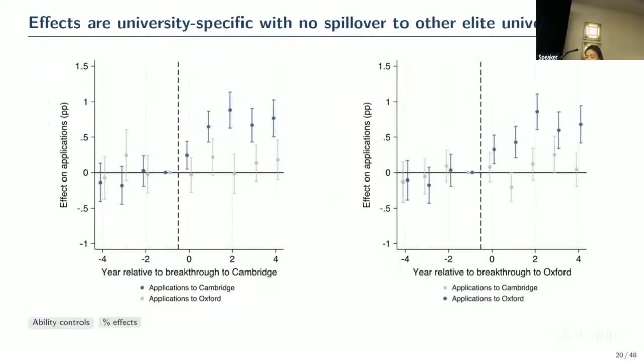
A Cambridge breakthrough raises later cohorts’ Cambridge applications by 0.6–0.8 percentage points, and an Oxford breakthrough raises Oxford applications by 0.4–0.8 points. Each lasts at least four years, and neither moves the other university (p. 14). Against the baseline application rate that is a rise of 30–50% (p. 2). The Oxford null was the fingerprint Tadjfar led with: what students learn is about one university, not “Oxbridge is for people like us.”

A questioner pointed out the problem straight away (00:19:36): you cannot apply to both Oxford and Cambridge in one year, so a Cambridge application is partly an Oxford non-application by construction. Tadjfar agreed it was “mechanical” and pointed to the stacked version; the paper’s Oxbridge discussion (pp. 14–15) does not mention the rule. The stacked result makes the case more cleanly. Pooling the top 10, applications to the breakthrough university rise 0.4–0.6 points, with no change in portfolios containing same-tier or higher-tier universities, and the new applications come out of lower-ranked ones (p. 15). With most applicants using all five ucas slots (80% in the paper, p. 7; “over 85%” in the talk), a breakthrough moves a slot up the ladder.

The induced applications are not wasted. Enrolment rises 0.3–0.4 points, 60–85% of the rise in applications, and the enrolment and graduation coefficients are nearly identical (pp. 15–16). For earnings the event study is underpowered (a 2SLS interval of roughly −£12,000 to +£92,000, fn. 17), so the paper matches. At 27, induced applicants earn £4,414 more than matched controls from control schools and £4,003 more than matched pre-breakthrough cohorts at the same school, about 15% of mean earnings (p. 16; the talk rounds both to £4,000). This is matching rather than a causal design, and “induced applicants” include always-takers (fn. 18). Asked what the counterfactual university was (00:27:23), Tadjfar said they had not ranked it yet but, from a Dale–Krueger (2014) exercise showing a premium concentrated at the very top, guessed it sits “in the 10 to 20 or 20 to 30 range” (00:28:24).

Effects are larger for students who resemble the breakthrough student: demographic overlap (low income, free school meals, gender) adds 0.1–0.25 points and social proximity (years at the same school, a shared subject) 0.5–0.75 (p. 17). Here the administrative data run out, as Tadjfar said herself: similar people are more likely to be friends, so this cannot separate co-location from information.

The harder objection was a university-specific school shock, such as a new teacher with a Cambridge connection or an outreach programme. Effects are not concentrated near the university, where outreach happens, and still appear for students sharing no subject with the breakthrough student, but the paper concedes the data cannot fully rule it out (p. 18); teacher-level data are coming through Vira’s ifs secondment. One questioner pushed further (00:24:54): test-score controls use averages when the action is in the narrow right tail, and four years of persistence needs a chain of students, which “speaks more from a school level shock” (00:25:47). Tadjfar replied that an ambitious teacher would probably push several universities, not one, and called teachers “a really important avenue for future research”. The questioner did not concede. (The model’s answer is the chain, each attendee renewing the good regime, but in school averages the two stories look alike.)

Manufacturing a breakthrough

The experiment covers 640 Year-13 students in 21 schools in England and Wales, randomised individually (p. 19). Everyone, controls included, got an hour-long workshop on admissions grades, earnings by university and the application process, so the treatment is exposure over and above general information. Treated students watched two three-to-four-minute videos of university students describing their school, grades, applications and social life, matched to the viewer’s academic tier. A video cannot become your friend, so a video effect is information, not co-location. Treated students were also re-randomised to up to two volunteer mentors from a pool of 245. T1 mentors share none of the student’s gender, ethnicity and home region, and T2 mentors share at least one; income is not among the matched traits (00:35:25). The intent-to-treat regression is (eq. 8, p. 23)

where $Y_i$ indicates applying to the student’s assigned video, mentor or any treatment university and $T_i$ is assignment to treatment, split into separate T1 and T2 dummies for the mentor comparison.

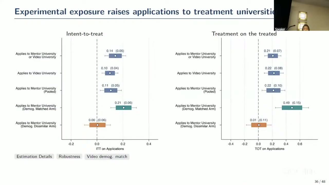
Pooled, treated students are 14 percentage points more likely to apply to an assigned treatment university (p = 0.004): 10 points for the video universities and 11 for the mentor universities (p. 23). That videos work as well as mentors is the paper’s argument against co-location. Then the split: a similar mentor raises applications to her university by 21 points (p = 0.001; 49 points on the treated), and a dissimilar mentor does essentially nothing (0.4 points, p = 0.952). Take-up was higher in the dissimilar arm, 42% against 35% (p. 24), so the null is not about disengagement. Tadjfar had just shown a mentor’s email (“keep the questions coming”, 00:33:47), and said “this is actually quite surprising because in the previous slide I showed you how engaged and intense that mentor interaction was” (00:35:04). (She described the tot as the itt “multiplied by a factor of two” because take-up was about 50% (00:34:28); in the paper the pooled ratio is 0.21/0.14, about 1.5.)

This is the most interesting result in the paper. The dissimilar mentor is just as real, at just as real a university, answering questions just as eagerly. What she cannot show the student is that someone like the student would be all right there, and that seems to be the fact that moves the application. (The appendix finds the video effects concentrated among students who share a speaker’s ethnicity or region too, though that match was not randomised.)

By ses, the effect is 17 points for low-ses students (p = 0.007) and 9 for high-ses students (p = 0.258) (p. 4). In the control group, low-ses students apply to their video university at 11% against 17% for high-ses students, and the treatment closes that gap (p. 25). Two caveats the talk did not mention: as of 9 September 2026, final application outcomes are in for 473 of the 640 students, 78 of them from endline self-reports rather than school records (fns. 24 and 33), and the preferred sample excludes students who said they did not want a mentor (pp. 22–23).

What the students believed

The belief data make this a paper about social fit rather than about role models. At baseline, controlling for predicted grades, low-ses students put their chance of fitting in and making friends at Oxford about 9 points lower than other students do (p = 0.001, p. 21), with no significant gap in their beliefs about getting an offer or graduating. They are also well calibrated on grades, and if anything optimistic: about 30% guess below Oxford’s 25th percentile (p. 22), which Tadjfar read as a sensible response to contextual offers.

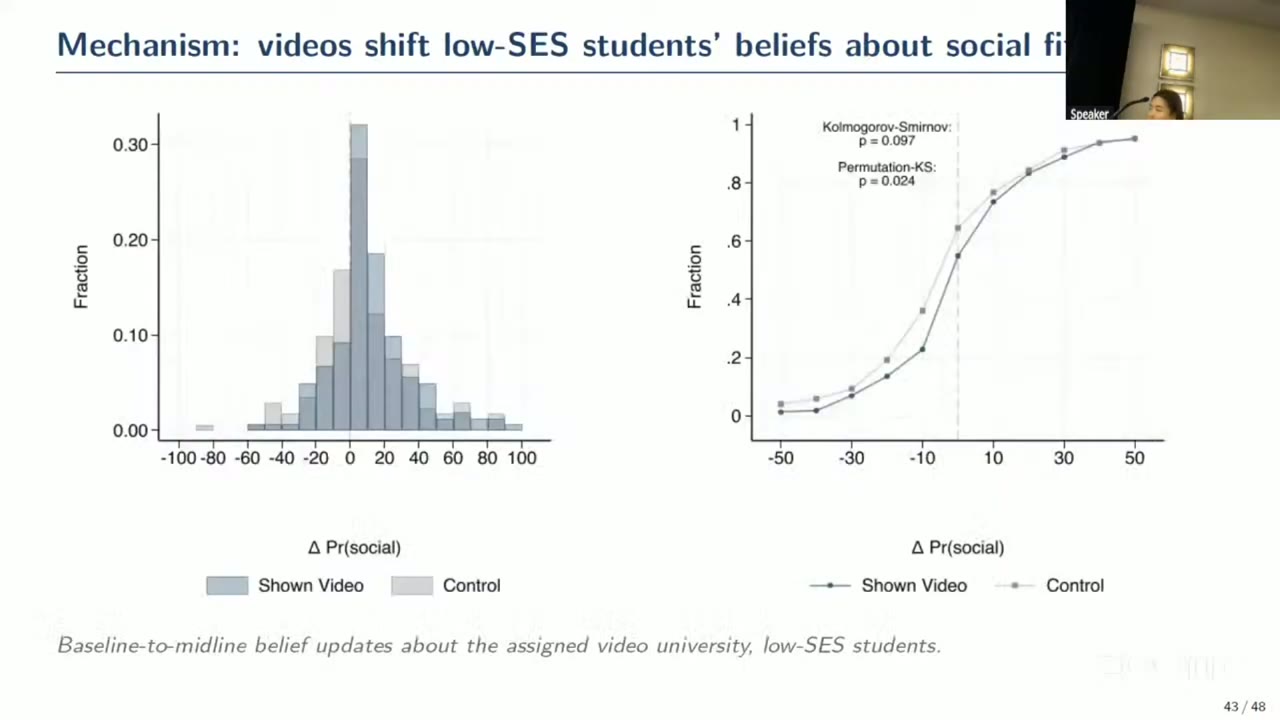
After the videos, low-ses students’ updates about fitting in at the video university shift right relative to control. The paper reports p = 0.024 (p. 25), which is the permutation ks test; the plain ks test on the same figure gives 0.097, and the figure notes don’t say which is which. For offers and graduation the permutation p-values are 0.732 and 0.386. High-ses students don’t move, and low-ses beliefs about Oxford, which no video featured, don’t move either.

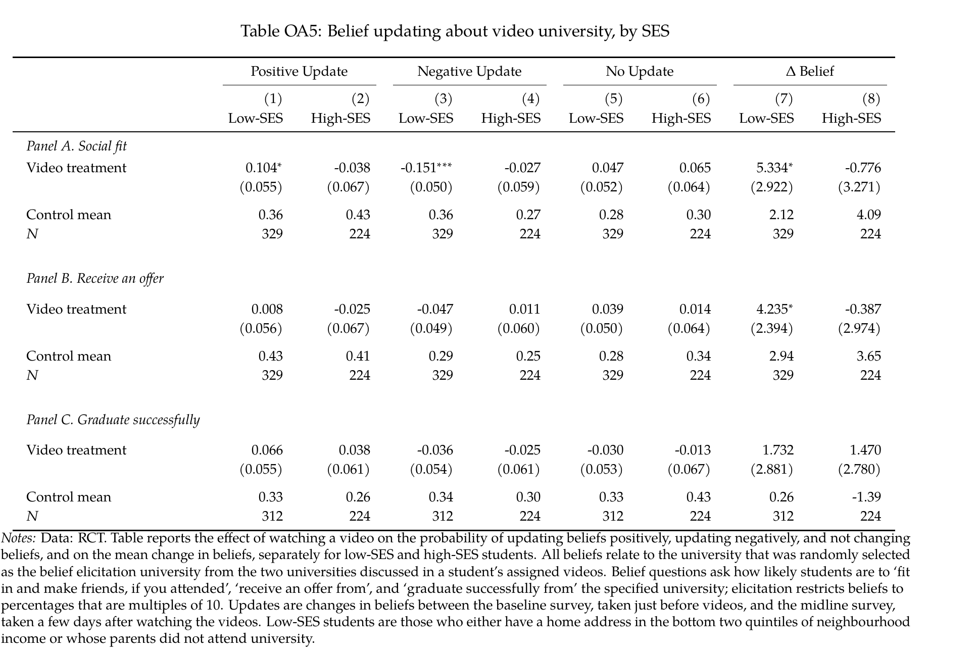
The regression version is less tidy than the talk. For low-ses students the video raises the probability of a positive social-fit update by 0.104 and cuts that of a negative one by 0.151, with the offer equivalents near zero. But the mean change in offer beliefs, +4.24, is nearly as large and as significant as that in social-fit beliefs, +5.33 (Table OA5, p. 52), and the text doesn’t discuss it. “Only social fit moves” holds for the distribution and the direction of updates, not for the means.

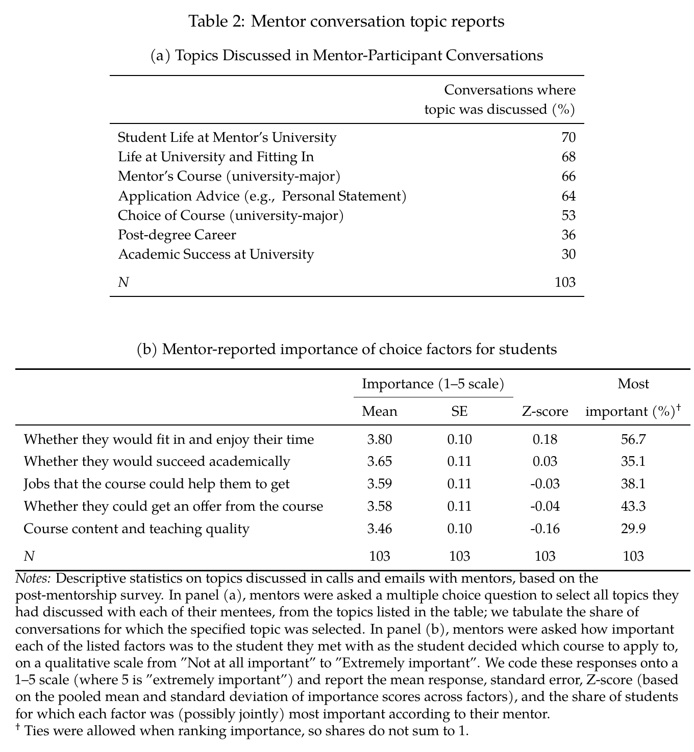
The mentor surveys point the same way, descriptively. In 103 conversations, student life came up in 70% and fitting in in 68%, careers in 36% and academic success in 30% (Table 2, p. 39). Mentors rated fitting in the most important factor in the student’s choice (3.80 out of 5; jointly top in 56.7% of cases). Of the careers figure, Tadjfar said “It’s shocking how … low that is” (00:42:32).

Role model or information

One questioner offered the obvious alternative (00:35:39): this sounds like a role-model effect, and with five slots a role model can hurt you, if you swap a safety school for a Cambridge application you won’t land. Tadjfar answered that the belief data look like information acquisition, and that in the administrative data students drawn in by breakthroughs get offers, graduate and earn more, so “we’re not really seeing evidence for like students just kind of throwing in applications and then losing a safety school” (00:36:21). A few minutes later she granted that “a role model effect is definitely at play here”, alongside the information (00:39:06). Earlier, a questioner seemed to ask whether the five-application cap was itself the friction (00:17:14; the question is garbled). She pointed to undermatching in the us and Chile: “it’s possible that’s suboptimal but … that’s kind of the world we’re in.”

Who’s to say

The policy point is that contextual offers lower the wrong bar. The uk has worked hard on the grades bar; the bar that binds is in the student’s head, and it is set by whether anyone from her school went last year. A few minutes of video, or a mentor who shares her gender, ethnicity or region, moves her application over and above the hour of grade distributions and earnings tables that everyone got.

What the paper cannot settle is whether the pessimism is wrong. “Maybe [low-ses] students are right to be pessimistic, right? Who’s to say?” Tadjfar said (00:42:32), and the experiment has no ground truth for social fit. The authors read the pessimism as excessive, and one of their two reasons is that breakthrough effects persist: if the breakthrough student had a terrible time, the effect should fade (p. 22). Their own Proposition 2 makes that weaker than it sounds. In the model any breakthrough outcome above $\bar x$, which is negative, still raises attendance, because watching someone go cuts uncertainty whatever she reports back. A mildly bad experience builds a pipeline too, so persistence rules out only quite bad ones. That leaves the beliefs that move after a video, and a 17-point effect on the students with the most to gain. It just means much of the evidence that these students are wrong about fitting in is evidence that they are unsure about it. Unsureness, it turns out, is the cheap part to fix.

References