Closing Small Open Economy Models

Stephanie Schmitt-Grohé and Martín Uribe, Journal of International Economics 2003. Read here in the November 2001 draft, whose numbers the published version carries over essentially unchanged. No talk recording exists; written from the paper alone.

There is a small embarrassment at the foundation of every small-open-economy business cycle model, and this paper is the field’s definitive piece of housekeeping about it. The embarrassment: take the most natural model you can write down — a small country whose households can borrow and lend at an exogenous world interest rate through a single risk-free bond — and it has no well-defined place to come back to. Its steady state depends on initial conditions. A transient productivity shock changes the country’s net foreign asset position permanently: the household, able to smooth consumption at a constant interest rate forever, has no reason to work its wealth back to any particular level, so consumption and foreign assets acquire a random-walk component and their unconditional variances are infinite. This is not an economic prediction anyone believes; it is a nuisance property that breaks the standard solution methods, which all work locally around a stationary point that the model declines to supply.

So the profession developed workarounds — small modifications with, as the authors put it with unusual candor, “no other purpose than to induce stationarity.” Every paper picked one, nobody was sure whether the choice mattered, and referees could always ask. Schmitt-Grohé and Uribe line up the five contenders, calibrate them identically (to Mendoza’s 1991 Canadian numbers, the next paper in this reading list), and race them.

Five ways to nail down a steady state

Each device works by making some equilibrium condition pin down consumption or debt in the steady state. An endogenous discount factor (Uzawa preferences) makes impatience rise with consumption, so the steady-state Euler equation β(c)(1 + r) = 1 solves for consumption directly. (A variant has the discount factor depend on aggregate rather than own consumption, which the authors note is “arguably no more arbitrary” and saves a state variable — a very economist form of honesty about how ad hoc the whole enterprise is.) A debt-elastic interest rate premium charges the country a spread that rises with its aggregate foreign debt,

so the steady-state condition β[1 + r + p(d)] = 1 pins down debt (this is equation 23 in the paper, and the device Neumeyer and Perri’s emerging-markets paper later in this list builds its whole economics on). Portfolio adjustment costs make it costly to hold debt away from a reference level, with a nearly identical log-linearization — the paper shows models 2 and 3 coincide to first order when ψ₂ = (1 + r)ψ₃, which in the calibration makes the two friction parameters come out at 0.000742 and 0.00074 respectively; note the size, of which more below. Complete asset markets tie home marginal utility to (exogenous, stationary) foreign marginal utility, which imports stationarity from abroad. And as a control, model 5 is the untreated patient: the nonstationary bond-economy itself, which still has impulse responses even though it has no unconditional moments.

The race is a nine-way tie

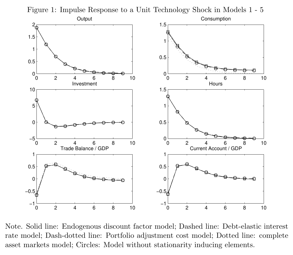
The result is in one picture, and it is the rare figure that is interesting because you cannot see anything: six panels of impulse responses to a technology shock, five models each, and “to the naked eye the graph appears to show just a single line.”

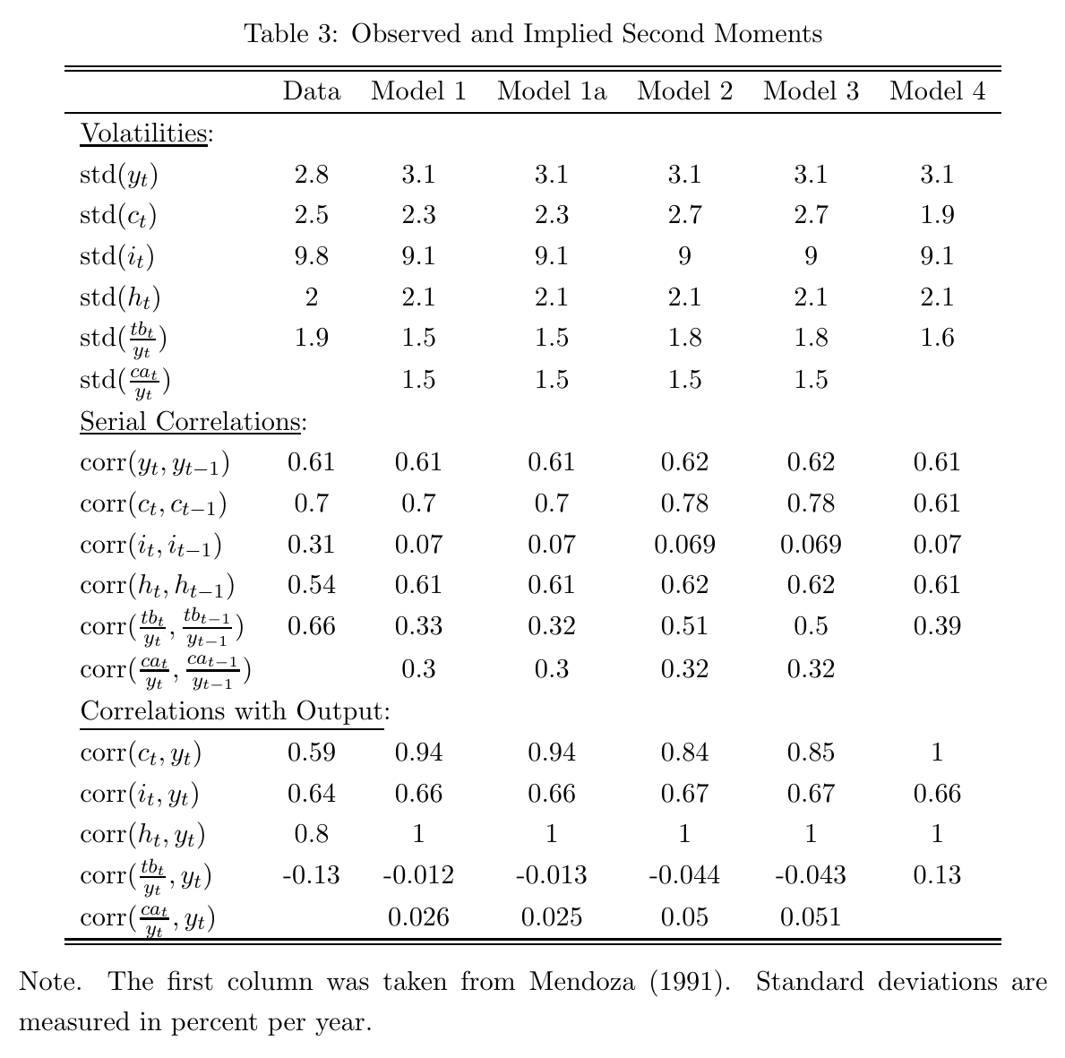
The second moments tell the same story: output volatility 3.1 percent in every model, investment volatility 9 to 9.1, hours 2.1. The one deviation is exactly where theory says it must be: under complete markets consumption is insured, so its volatility drops (1.9 against 2.3–2.7 in the incomplete-markets versions) and the trade balance flips from mildly countercyclical to mildly procyclical (+0.13 against −0.01 to −0.04).

Why the tie? Because the friction parameters needed to do the job are tiny — a debt-premium coefficient of 0.000742, calibrated to match the volatility of the Canadian current account. The devices operate at frequency zero: they anchor where the economy drifts over decades while leaving the business-cycle mechanics — the intratemporal labor condition, the capital Euler equation, the response to a persistent productivity shock — untouched. The random walk they remove was always a low-frequency pathology, so its cure is a low-frequency intervention.

The license, and its fine print

The paper’s conclusion is a license the field has been citing ever since: if your reason for the modification is “simply technical,” pick whichever is computationally most convenient. (The original Uzawa specification loses on those grounds — it drags an extra state variable and Euler equation around. The debt-elastic premium won the popularity contest.) Even the complete/incomplete markets choice barely matters for aggregate dynamics, echoing Kollmann and Baxter–Crucini in two-country settings — and rhyming, from the other direction, with BKK’s finding earlier in this list that shutting trade down entirely changed little. There is a pattern here: in frictionless-ish real models, the market structure keeps failing to matter, which is either reassuring or a hint that these models are missing whatever makes it matter.

The fine print is what happens when the reason is not simply technical, and the rest of this syllabus is largely a tour of that fine print. If the interest rate premium is not a 0.0007 technicality but a large, volatile object with its own shocks — Neumeyer and Perri’s Argentina — it stops being a closing device and becomes the engine. If borrowing constraints arise endogenously from default risk — the Eaton–Gersovitz tradition, Restrepo-Echavarría’s limited-commitment work — the “device” is the economics. This paper is the hinge between those two readings: it establishes precisely the sense in which the closing device is innocuous, which is exactly what lets later papers claim, when they load economics onto the same object, that the action is coming from the economics and not the plumbing.