Sanctions and the Exchange Rate

Oleg Itskhoki (Harvard University) and Dmitry Mukhin (London School of Economics), “Sanctions and the Exchange Rate”, Review of Economic Studies (2026) 93(4): 2680–2714, advance access 27 September 2025, editor Kurt Mitman — the published version is the version of record used throughout, superseding NBER Working Paper 30009 of May 2022 (a short version of which appeared in Intereconomics 57(3)). Presented by Itskhoki at Markus’ Academy, the Princeton Bendheim Center webinar, on 24 June 2022, hosted by Markus Brunnermeier, with no discussant. The talk was given on the working paper, so every proposition, equation and figure number Itskhoki says aloud is the working paper’s, not the published one. Figures 1, 4, 5, 6 and Table A1 are crops from the published version; the Swiss-franc exhibit is a crop from the 2022 working paper.

The best-performing currency of 2022

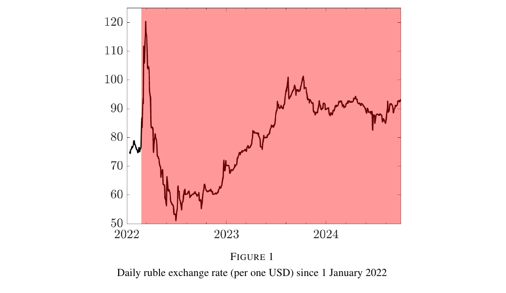
The ruble was at 75 to the dollar when Russia invaded Ukraine on 24 February 2022. It lost half its value within days, was back at its pre-war level a few weeks later, and by June had appreciated another 30% — a seven-year high, reached while the number of sanctions on the country only went up. Krugman wrote about “The Curious Case of the Recovering Ruble”; Guriev called it “The Incredible Bouncing Ruble”. Itskhoki and Mukhin’s answer, in 2022 and again in the published version, is that there was never a puzzle. A standard model of exchange-rate determination in a small open economy, with one unusual ingredient, produces the crash and the over-appreciation from the sanctions that were actually imposed, and it delivers a warning on the way out: the exchange rate is not a sufficient statistic for whether sanctions are working, and in the spring of 2022 it was pointing the wrong way.

A currency market with two sides

You are a household in a country whose banks have just been cut off from the rest of the world. You cannot lend abroad; nobody abroad will lend to you. The only agents who can move money across the border are the government, the state banks and the exporting companies, which the published version folds into a single government sector. So the foreign currency available to you arrives from exactly two places — commodity export revenue and whatever reserves the central bank chooses to sell — and it goes to exactly two places, the imports you buy and the dollars you decide to sit on. The exchange rate is the price that clears that market. That is the whole model, and it is worth noticing how much of the standard apparatus it does without.

The published version commits to functional forms the working paper left general: preferences are CES with elasticity $\theta > 1$ between home and imported goods, plus a quadratic bonds-in-utility term $v(b;\Psi) = -(\kappa/2)(b-\Psi)^2$, both in equation (3) on p. 2685. Readers of the old draft should know that the Cobb–Douglas case — the one that yielded a tidy closed form for the exchange rate — has been explicitly relegated to the working paper (footnotes 9 and 16, pp. 2685 and 2691), and with $\theta$ now free the closed form is a pair of equations rather than one. The unusual ingredient survives, in the household Euler equation for foreign-currency bonds, equation (6), p. 2687:

Here $B^*_{t+1}$ is household foreign-currency savings, $R^*_{Ht}$ the return they are actually allowed to earn on it (possibly repressed below the world rate $R^*_t$), and $\Psi_t$ a shock to the desire to hold foreign currency as a safe asset regardless of return — a precautionary demand, which is what a collapsing stock market, a bank run and foreigners unwinding their positions look like when you write them down as one variable.

The rest is bookkeeping, and the bookkeeping is the result. In the stationary case the country budget constraint fixes the imports the economy can afford, and the import demand schedule then reads off the exchange rate that supports them — equations (10) on p. 2689 and (12) on p. 2691:

$\mathcal{E}_t$ is the nominal exchange rate in rubles per dollar, $P_t$ the domestic price level, $C_{Ft}$ imports, $Q^*_t X_t$ commodity export revenue at world prices, and $F^*_0$ the country’s net foreign assets. Sanctions that hit the numerator of (12) — export prices, export quantities, or the assets themselves — make foreign currency scarce and depreciate the ruble. Sanctions that raise the import price $P^*_t$ shrink $C_{Ft}$ by exactly as much, but appreciate the ruble through (10), because at $\theta > 1$ dearer imports mean less spending on imports and therefore less demand for dollars.

The same pain, opposite signs

Proposition 1 (p. 2688) makes the equivalence exact. Permanent import sanctions of size $\tau$ deliver the same path of imports and the same welfare as permanent export sanctions of size $\tau$ combined with a proportional seizure of foreign assets — the asset seizure being necessary because net foreign assets are the sufficient statistic for past trade imbalances, and dynamic Lerner symmetry requires uniformity across periods, which means taxing the accumulated proceeds of past exports too. The export-cum-seizure package simply depreciates the currency by an extra $\tau$ percent along the way. Proposition 2 (p. 2690) puts numbers on it through equation (11): a permanent depreciation of $\tau/\theta$ under export sanctions against a permanent appreciation of $((\theta-1)/\theta)\tau$ under import sanctions, plus, when $\kappa > 0$, an additional transitory depreciation in both cases as households rebuild the foreign savings the sanctions destroyed. Readers of the working paper will find these renumbered: its separate propositions on export and import sanctions are now Propositions 1 and 2, its Lerner result is split across Propositions 1 and 3, and its result that a shrinking domestic endowment appreciates the currency has been demoted to a footnote (fn. 18, p. 2693) because the quantitative section finds that channel small.

The genuinely uncomfortable result is Proposition 3 (p. 2692). The equivalence extends past the allocation to the fiscal balance, the consumer price index and the real cost of living, with equation (14) giving the losses as $\hat{TR}_t = -\chi_t((\theta-1)/\theta)\tau$ and $\hat{\mathcal{P}}_t = \mu_t(\tau/\theta)$, where $\chi_t$ is the export share of revenues and $\mu_t$ the import share of expenditure. Import sanctions reduce government revenue by exactly as much as export sanctions even when literally all tax revenue is collected on exports and none on imports, because the appreciation they cause shrinks the local-currency value of every barrel sold; export sanctions raise consumer prices by exactly as much as import sanctions even though they touch no import price, because the depreciation they cause does it. The exchange rate is not the thing that happens to sanctions. It is the thing that makes both kinds of sanctions land in the same place. Brunnermeier polled the audience on this before the talk: 53 percent thought that sanctioning imports rather than exports made the war easier for Russia to finance, 21 percent thought the two equally effective, 26 percent said it did not matter for the short-run deficit [00:05:19]. The paper’s answer is the 21 percent, and Itskhoki conceded on the call that this is not intuitive until you notice that export revenue only matters through what it can buy.

The equivalence has honest limits, set out in Section 2.2.3 (pp. 2694–95): it needs sanctions to be permanent and unanticipated, it fails for temporary or pre-announced measures, and a depreciation can bite harder than an appreciation in a dollarized economy through balance sheets — which, the authors note, was irrelevant for Russia in 2022, since after 2014 it had no net foreign-currency debt (fn. 23, p. 2695).

Why the first month looked different

Now switch on $\Psi_t$. In normal times a central bank meets a precautionary rush into dollars by selling reserves, and Proposition 4(a) (p. 2695) says this is not merely adequate but welfare-maximizing: imports, the exchange rate and net foreign assets do not move at all, because reserves and household savings are the same country’s dollars in different pockets. Freeze the reserves and that option is gone. The government can then be passive — Proposition 4(b) and Figure 3 on p. 2697 — in which case households fund their hoarding by cutting imports, and the currency takes a jump depreciation that unwinds only as the savings are rebuilt. Or it can repress: tax the purchase of foreign currency, force exporters to surrender their revenue, cap transfers abroad. Proposition 4(c) says repression leaves imports, the exchange rate and the asset path exactly where full accommodation would have left them, and charges the entire bill to savers. Russia did the second. Exporters were made to surrender 80 percent of their foreign-currency revenue, later cut to 50; transfers abroad were capped at $5,000 [01:10:24]; dollar purchases were taxed at 12 percent.

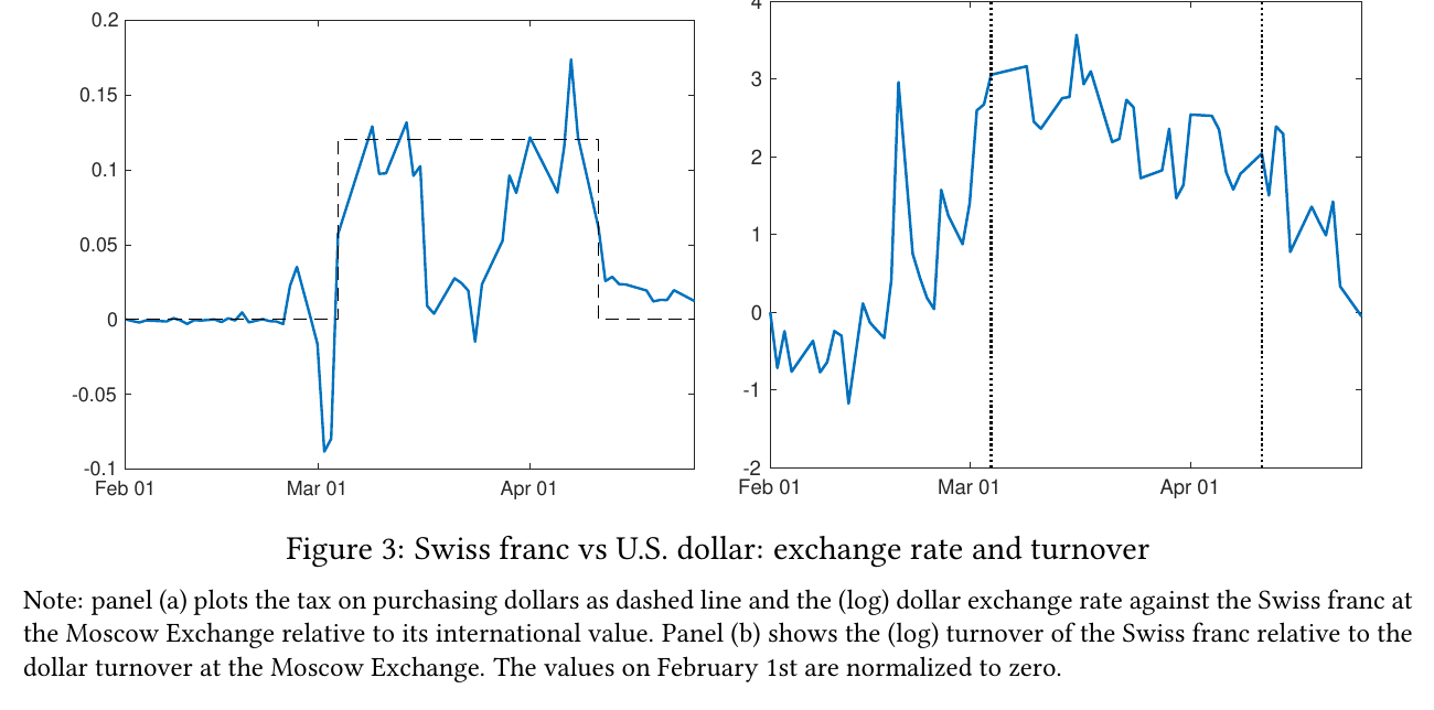
The 12 percent tax produced the episode Itskhoki clearly enjoyed most. It applied to dollars, euros and pounds, and — because Switzerland had not yet joined the sanctions when the rule was drafted — not to Swiss francs. So the franc–dollar rate quoted in Moscow departed from the world franc–dollar rate by exactly the tax, for exactly the duration of the tax, and franc turnover rose three- to four-fold before everyone went back to dollars [01:11:06–01:12:29]. It is as clean a demonstration as one could ask that these are market prices responding to a wedge, and the published version dropped it, keeping only an allusion in footnote 28 on p. 2697. The exhibit below is therefore the working paper’s, and the working paper’s alone.

Repression is welfare-reducing in a representative-agent economy, which raises the question of why every government reaches for it. The published version’s answer, now an unnumbered discussion on p. 2698 and Appendix C.2 rather than the working paper’s Proposition 6, is redistribution: repression takes foreign currency away from the few who want to hoard it and leaves it for the many who would spend it on imports, so with enough hand-to-mouth consumers a utilitarian planner can like it.

The sanctioner’s side, which is new

The working paper stopped roughly there. Section 3 of the published version (pp. 2698–2702) builds out the rest of the world as a real economy that consumes commodities, and finds that Lerner symmetry survives the trip: Proposition 5 (p. 2699) shows a permanent import tariff $\tau$ is equivalent to an export tax $\tau$ plus a seizure of $\tau/(1+\tau)$ of foreign assets, with equation (19) giving the transfer that accrues to the sanctioning coalition. This has immediate policy content. A price cap set at $1/(1+\tau)$ of the world price replicates the export tax exactly (p. 2700), which is the theoretical case for the instrument the G7 actually chose. Quantity restrictions are worse, and instructively so: with inelastic export supply they slide up the world demand curve instead of down the supply curve, so world prices rise, the rents go to whoever controls distribution rather than to the coalition, the rest of the world loses outright, and the target loses export revenue only if $s_t/\eta < 1$ (p. 2701). And coalitions leak — equation (20) shows that a coalition covering only a fraction $\delta$ of import varieties with substitutability $\rho$ needs ever larger individual tariffs to deliver a given uniform-equivalent tariff, and for a homogeneous good, as $\rho \to \infty$, only a complete coalition does anything at all (p. 2702).

The forecast that came true

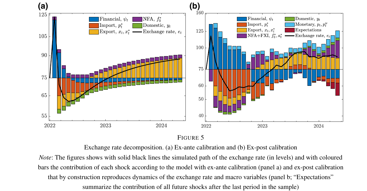
Section 4 (pp. 2702–10) is the other new half: a monthly quantitative model run from February 2022 to September 2024, with $\beta = 0.96^{1/12}$, $\theta = 1.5$, $\bar\kappa = 0.33$, $\gamma = 0.25$ and commodity demand elasticity $\eta = 0.05$ (p. 2703). It comes in two calibrations, and the difference between them is the best thing in the paper. The ex-post calibration backs the shocks out of the data, including $\psi_t$ as the residual that fits the exchange rate exactly, and then validates that residual against euro interest-rate spreads and gross capital outflows it was not fitted to (Appendix E, p. 2707). The ex-ante calibration reproduces what the authors wrote down in September 2022, on the scraps of information available then, targeting not a single exchange-rate moment.

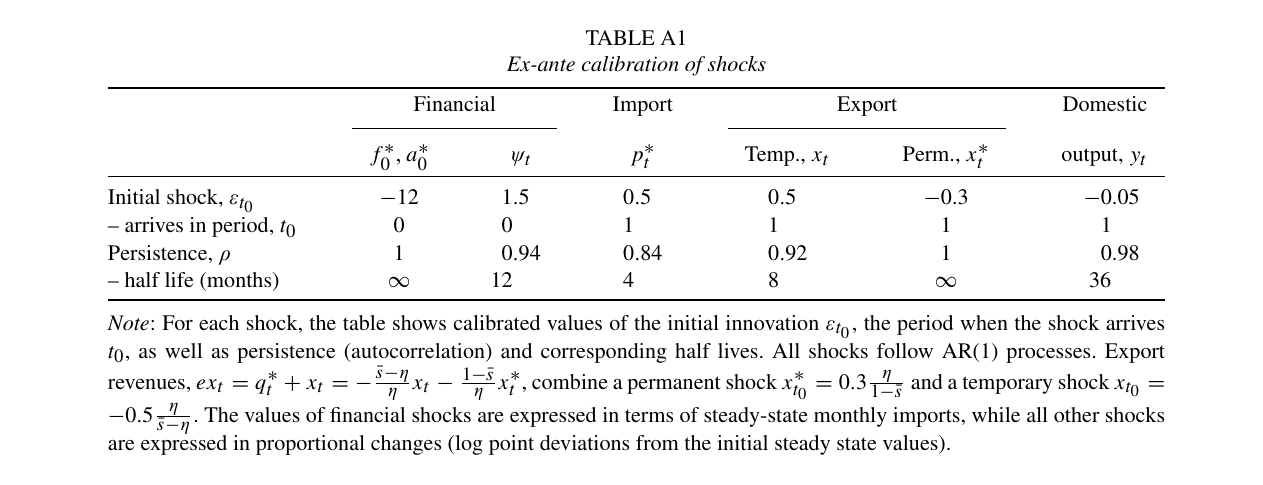
The inputs are the headlines of the first weeks. About half of Russia’s foreign assets, some $300 billion, were frozen in week one, which is a permanent reduction in $f^*_0$worth twelve months of imports; the panic is$\psi_0 = 1.5$months of imports with a one-year half-life, cross-checked against the$20 billion rise in household foreign-currency cash and the $100 billion foreigners pulled from Russian bond and equity funds in February and March (fn. 35, p. 2703). Imports fell from $30 billion a month to $17 billion in April and recovered to $24 billion by mid-summer, entered as a 50 percent import-price shock with a four-month half-life; export revenues rose from $35 billion a month to $50 billion (fn. 36, p. 2704), entered as a temporary 50 percent increase against a permanent 30 percent decline; output falls 5 percent; everything non-financial arrives with a one-month lag (p. 2703).

Out of this the model depreciates 50 percent on impact, returns to the pre-war level in about a month, peaks 20 percent stronger at the four-month horizon, and — this is the part written in September 2022, with the ruble still conspicuously strong — predicts a return to the pre-war level around February 2023 and a long-run rate of 92 to the dollar. The ruble came back on schedule. It has since settled around 95, against a pre-war 75 (p. 2705 and fn. 38). The model misses the swings around the Wagner mutiny in the summer of 2023, which is the sort of thing a model of currency supply and demand should miss.

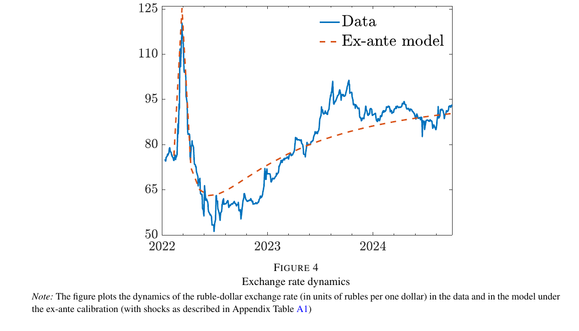
The decomposition says who did what. The financial shock drives the first weeks, and the ex-post calibration finds the depreciation would have been 10 percent larger had the central bank not sold reserves into it (p. 2705). The $300 billion freeze itself, taken alone, is worth a permanent depreciation of 3 percent — an asset stock equal to a year of exports is about 4 percent of export flows at the annual interest rate, and that is all a permanent income loss of that size can do to a price. Its real effect was indirect, in disabling the intervention that would have absorbed the panic. From month one the trade shocks take over, from month three they appreciate the currency, and then parallel imports reopen while export revenues fall, which brings the ruble back to pre-war about a year in and roughly 20 percent weaker thereafter.

What it cost, and to whom

The initial depreciation boosted local-currency fiscal revenues by 12 percent, which is the mechanical reason a finance ministry may prefer a weak currency to a strong one. Net of the monetary inflation that builds to 20 percent over the sample, real revenue turns negative from April 2022 onward, and excluding the domestic output collapse — which mostly mirrors war spending — sanctions reduce long-run real government revenue and national income by about 4 percent (p. 2708). The authors work with the consolidated budget throughout, noting that energy exports are a disproportionate 40 percent of the federal budget against a 25 percent share of GDP (fn. 39, p. 2707). On the household side, consumption losses over the sample run to 7 percent from import sanctions, 1.8 percent from export sanctions net of the early commodity windfall, and 0.6 percent from the asset freeze combined with the reserve movements; two and a half years of this is equivalent to a permanent 0.9 percent decline in consumption, which the authors observe is “vastly larger than the conventional estimates of the cost of a business cycle” (p. 2708).

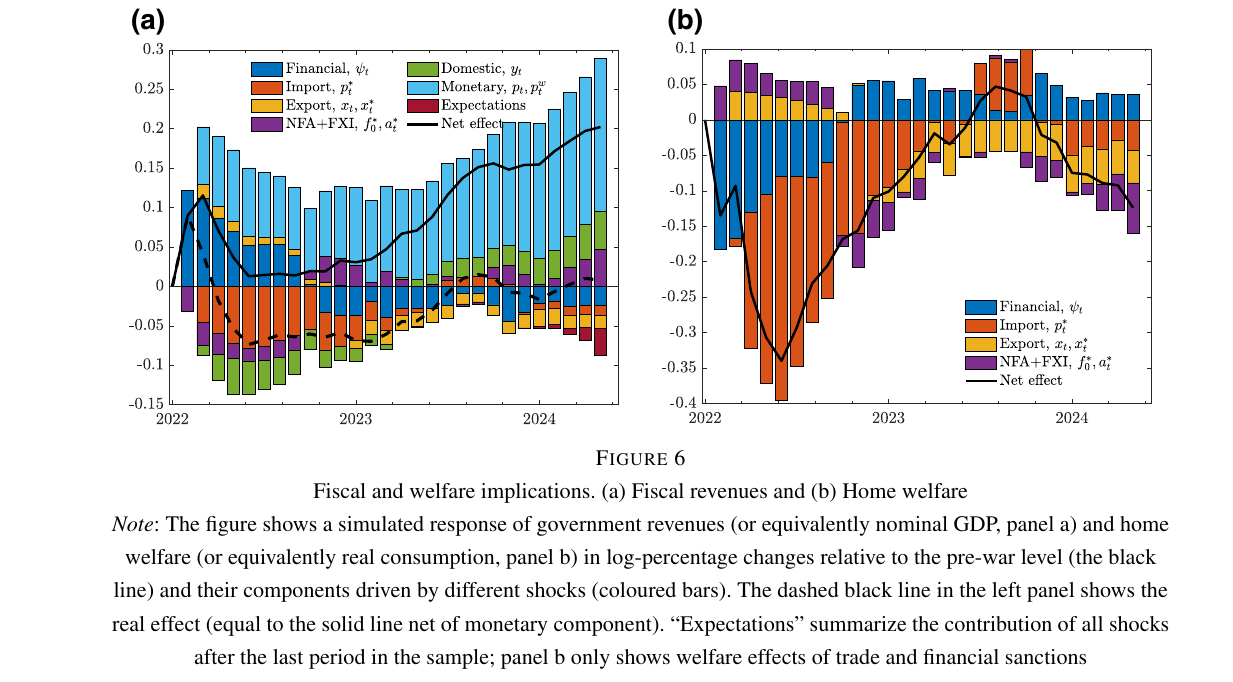
For the coalition, the arithmetic is less flattering than the rhetoric. Freezes, tariffs and financial shocks are transfers, and they are worth about 0.2 percent of annual consumption to the sanctioners. Quantity-type export sanctions are not transfers, and they raised foreign consumer prices by about 1 percent in the first months — roughly half of overall inflation in that window — before dissipating in 2023 as the world energy market substituted. Netted out, the effect of all the sanctions on the rest of the world is close to zero (pp. 2709–10), before counting the direct costs of the war, which the model does not.

What the audience pushed on

Brunnermeier asked when the equivalence breaks, and proposed his own answer: if the exchange rate is used as a signal — of strength to one’s own population, of the likelihood of a bank run — then it becomes a goal in itself rather than a price, and the two sanction packages stop being interchangeable in the only dimension anyone is watching. Itskhoki agreed, and located it outside the model [01:04:34]. Asked where the ruble would be at year-end, he took the random-walk position, then listed the forces for depreciation — budget pressure, shadow import channels reopening, the EU oil embargo due in December — and said “it will revert back to 75 basically” [01:16:41–01:18:07]. Published Figure 1 shows that it did, about six months later than he suggested and then kept going. Asked whether the exchange rate is worth caring about at all, he was blunt: “it’s an allocatively relevant variable… what you can read off from the data is that sanctions are actually working” — the composition was simply heavy on imports [01:18:21]. From the floor: no meaningful black-market rate emerged once the depreciation pressure ceased [00:14:48]; demanding payment for gas in rubles merely moves euros “from the pocket of Gazprom to the pocket of the central bank” and does nothing in the model [00:39:21]; and yes, multiple equilibria are possible, and a government with instruments will pick the calm one [00:22:58].

Where it sits

This is the exchange-rate accounting of sanctions on the target, and the mirror of Bianchi and Sosa-Padilla’s work on the sanctioner’s side. Lorenzoni and Werning’s minimalist ruble model is its contemporaneous twin, now published in AER: Insights 5, 347–356 (2023), and the published version cites it in the main text (pp. 2684, 2691), crediting it with the goods-market route to the same appreciation result. Itskhoki and Ribakova’s survey has likewise landed, in Brookings Papers on Economic Activity, Fall 2024, 425–470. The authors state their own contribution as extending Lerner symmetry to a fully dynamic macro environment and then going past it quantitatively (p. 2684), and they point to Eichengreen et al. (2023) and Krahnke et al. (2024) for historical evidence that the predictions hold outside 2022.

The working paper was a note: two equations, a handful of comparative statics, and a correction to a misreading of the data. The published version is not. It has an optimal-tariff model of the sanctioning coalition, two independently disciplined calibrations, a validation exercise, and welfare, fiscal and inflation accounting for both sides of the sanctions. It is now the quantitative benchmark for the ruble episode rather than the accounting identity behind it. The gotcha it contributes is unchanged and stated in its own conclusion: the currency is not a scoreboard. In the spring of 2022 a great many people read a strong ruble as evidence that sanctions had failed, when what the model says a strong ruble measures is how much of the sanctions fell on imports — which is to say, on the thing Russian households were going to be denied either way.