Purifying the Equity Premium

“Purifying the Equity Premium,” by Christopher Polk (London School of Economics) and Tuomo Vuolteenaho (Arrowstreet Capital), presented by Polk at the NBER conference on New Developments in Long-Term Asset Management, Chicago, 18 April 2026. There was no discussant, and the recording carries no questions from the floor. Written from the June 2026 FMG draft.

What, exactly, are you comparing stocks to?

Start small. You own stocks, and you would like to know what you are being paid for owning them instead of something safe. To answer that you need the safe thing. Everyone — textbooks, practitioners, seventy years of asset pricing — uses the three-month Treasury bill, and defines the equity premium as stocks minus bills.

Now make the phrase “risk-free asset” say what it literally means. A three-month bill is risk-free in the sense that in three months you will receive a known number of dollars. That is a very specific promise, and it is only impressive if a known number of dollars three months from now is the thing you want. Stocks promise something else: an unknown stream of real cash flows, forever. So the conventional equity premium nets a real claim with a duration measured in decades against a nominal claim with a duration of one quarter. Polk, in the first minute of the talk, calls this “an apples-to-oranges comparison”: “stocks are real assets, and the T-bill is nominal… stocks are long-lived assets, and of course, the T-bill is explicitly short-term.”

Fix the mismatch and something falls out of it. Build the asset a long-horizon investor would actually call safe — a long-dated inflation-indexed bond, levered until its sensitivity to real rates matches the stock market’s — and call its excess return over bills the real term premium. Whatever is left when you subtract that from the conventional premium is the pure equity premium: the compensation for bearing dividend risk and nothing else. The arithmetic is arranged so that nothing at all is estimated in the split,

where $\text{SCALE}$ — stock duration over real-bond duration — is fixed at the start of each month, so this is an implementable portfolio and not a hindsight construct. The only judgement calls are how you measure the two durations. Which, it turns out, is where all the trouble is.

How long is a stock?

You cannot buy a fifty-five-year TIPS, because none exists. So you buy the longest inflation-indexed bond outstanding — a TIPS in the United States, an index-linked gilt in the United Kingdom — and lever it, borrowing at the bill rate, until its price sensitivity to a parallel move in real yields equals the stock market’s. This matches first-order price sensitivity; it does not move the bond’s cash flows further out. The portfolio rotates into whatever bond is longest at the time, which is why the duration line steps up in jumps: “You can see it jumps when we move into the longest maturity bond.”

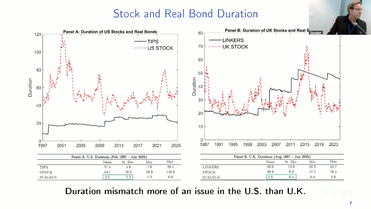
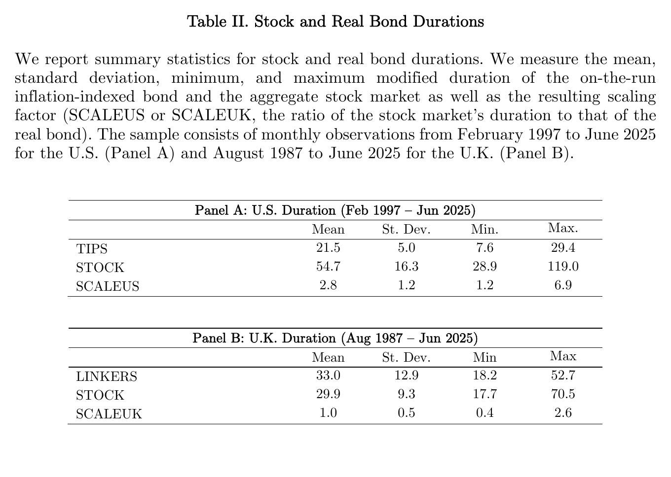
Stock duration is not estimated by regression. Under the Gordon growth model the modified duration of a stock is just its price divided by next year’s dividend — the inverse of the forward dividend yield — and the paper proxies that with the trailing twelve-month yield. Over the U.S. sample this averages 54.7 years against 21.5 years for the longest TIPS, so the bond leg has to be levered 2.8 times on average. That 54.7 is a sample mean, not a reading for today; the series is highly variable and touched 119 years at the dot-com peak. The United Kingdom is the methodological gift here: long Linkers are long enough that U.K. stock duration (29.9 years on average) and Linker duration (33.0) nearly coincide, and the scale factor averages 1.0. Whatever you think of levering a TIPS by 2.8, you cannot think it about the U.K. results, where the leverage is, in Polk’s phrase, “basically just sort of fine-tuning.”

The split

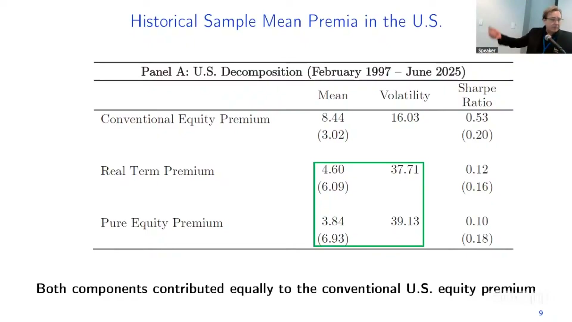
Over February 1997 to June 2025 the conventional U.S. equity premium ran at 8.44% a year. Split it, and the two halves come out at 4.60% for the real term premium and 3.84% for the pure equity premium: roughly half of the famous number was a levered bet on the long end of the real curve. In the United Kingdom, over a longer August 1987 sample, the conventional premium is a miserable 3.02% a year, of which about three quarters is the bond leg and 0.75% is the equity part. The paper’s own summary of that is admirably flat: “Taking on dividend risk simply did not pay off at all in the U.K. over that time.”

The surprising thing

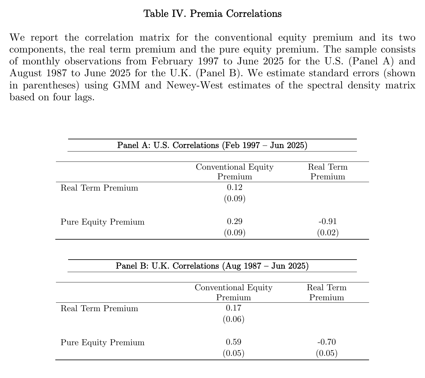
Here is the part that should stop you. The means split roughly in half. The volatilities do not. The real term premium realized an annualized volatility of 37.71% and the pure equity premium 39.13% — each of them more than twice the 16.03% volatility of the whole thing they add up to. Two series sum to a third series that is less than half as volatile as either of them. That is arithmetically possible only if they are violently negatively correlated, and they are: the measured correlation between the pure equity premium and the real term premium is −0.91 in the United States and −0.70 in the United Kingdom.

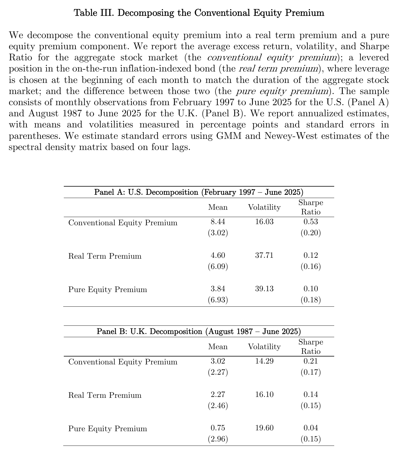
So the thing the profession has been measuring and puzzling over since Mehra and Prescott is the small, quiet residue of two enormous trades that very nearly cancel. Its celebrated Sharpe ratio of 0.53 is in part a diversification outcome — what you get when you net two offsetting positions, not what you get from a single richly compensated risk. Of the six full-sample Sharpe ratios in that table, only the conventional U.S. one is statistically distinguishable from zero; the components’ own ratios, 0.12 and 0.10, are noise at these sample lengths.

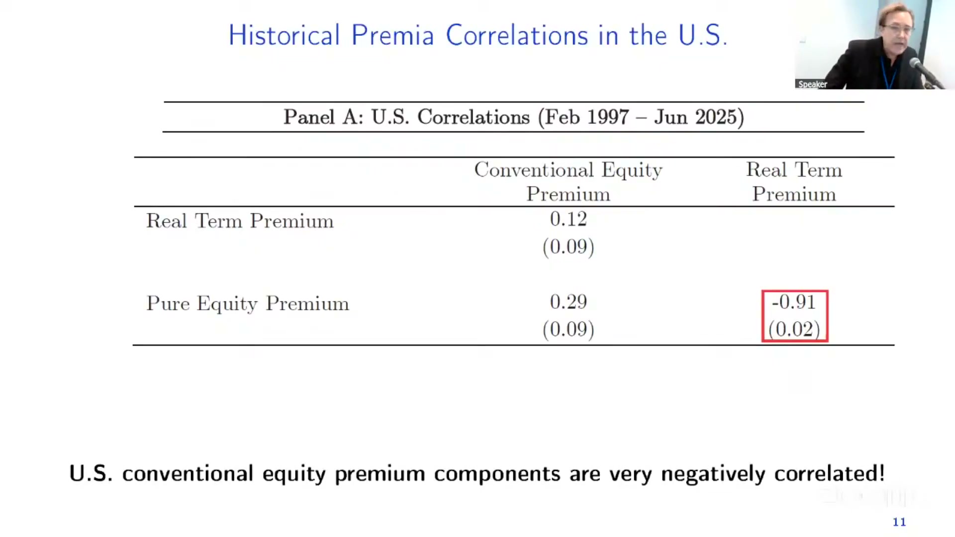
The first casualty is an entire measurement literature. If you have ever estimated equity duration by regressing stock returns on bond returns, the pure equity premium is your omitted variable, and it is not a nuisance — it is larger than your signal and correlated with it at −0.91. The paper’s verdict is unusually blunt for a finance journal: “one can simply say farewell to any hope of measuring stock market cash-flow duration from a simple regression of stock returns on bond returns.” There is also a circularity, which is the deeper reason: to compute the pure premium at all you must first take a stand on duration.

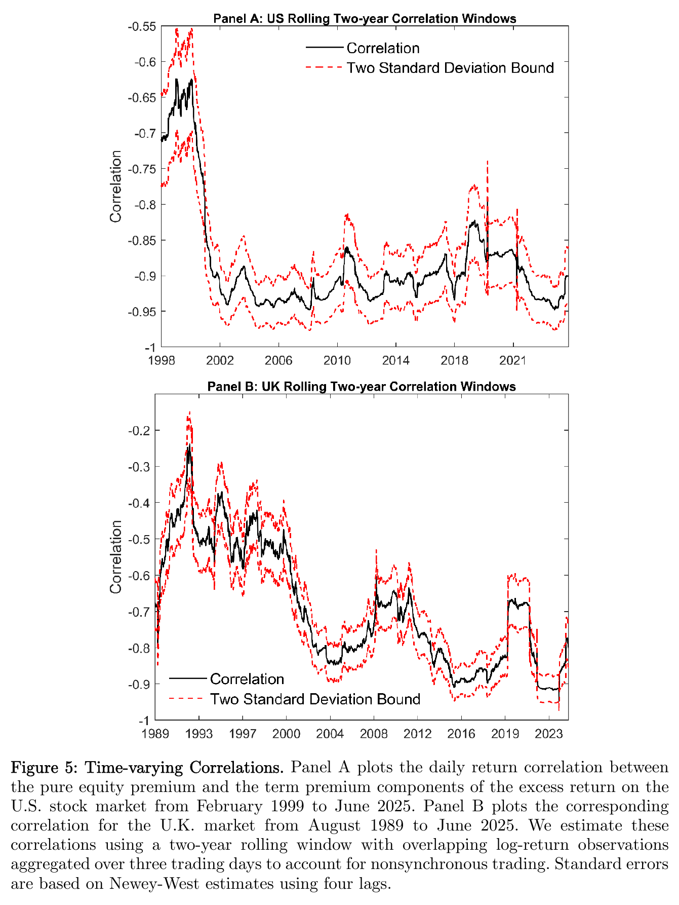
And it is not one crisis doing the work. Rolling two-year correlations estimated from daily data stay deep in negative territory throughout both samples, with the upper two-standard-error band never approaching zero. In the talk: “though there is some variation perhaps, it’s always deep in negative territory. Always statistically significant.”

Is it news about dividends?

The obvious story is that some fundamental shock hits, and it drives both legs: bad cash-flow news raises equity risk premia through habit formation and lowers real rates through precautionary saving. Call it the cash-flow hypothesis. The alternative is that preference shocks unrelated to fundamentals push forward-looking equity risk premia and real term premia in opposite directions — flight to safety, arising endogenously rather than from anything happening at the companies.

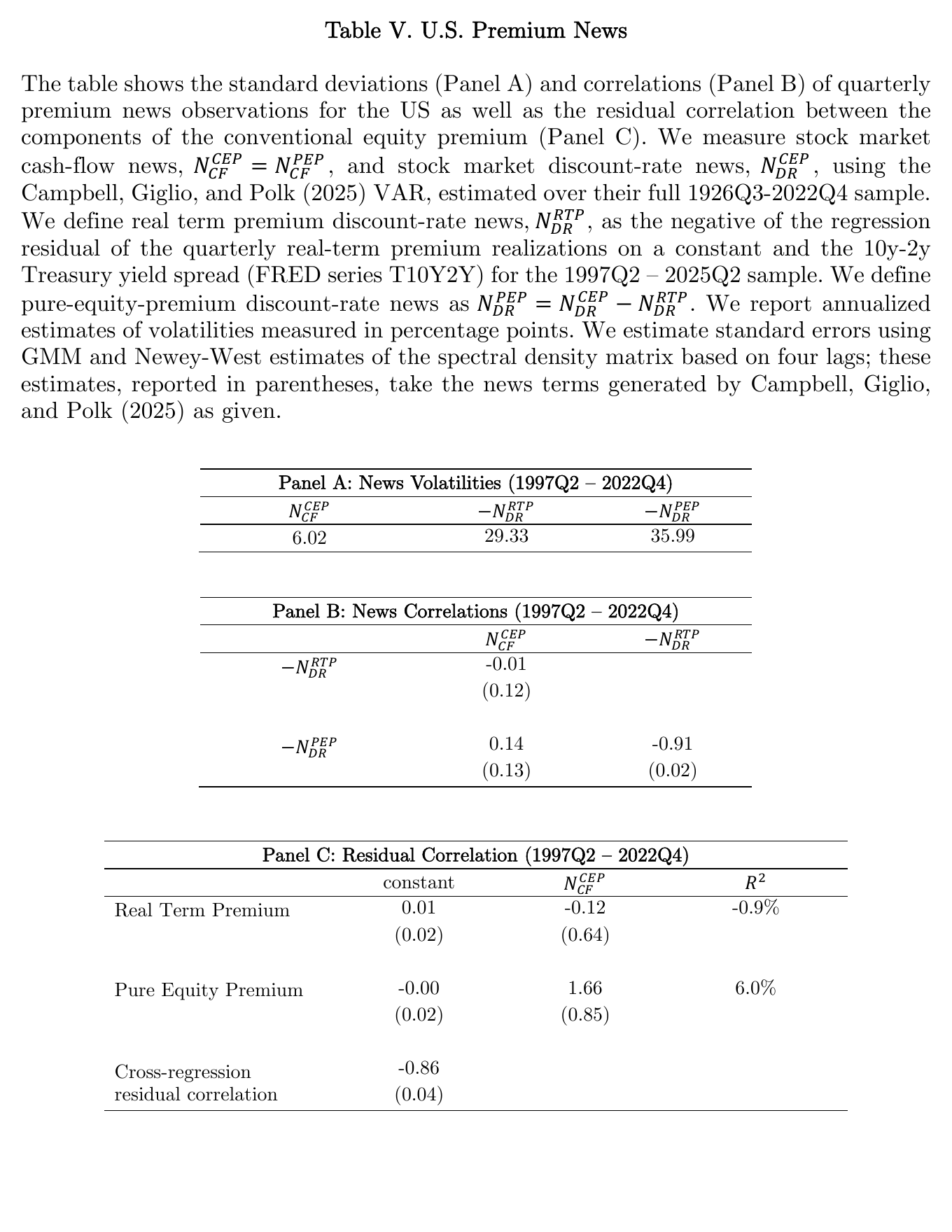
Using the Campbell–Giglio–Polk quarterly VAR to extract cash-flow news, the paper finds that measured cash-flow news is tiny beside either discount-rate term (annualized volatility of 6.02% against 29.33% and 35.99%), is essentially uncorrelated with the real term premium’s discount-rate news, and explains almost none of either realized component. Purge both series of cash-flow news and their residuals still correlate at −0.86. The paper’s own register is careful, and worth preserving: it reads this as “unsupportive of the cash-flow hypothesis” and concludes that “we cannot trace the very negative correlation between the pure equity premium and the real term premium to stock market cash flows.” That is not the same as ruling cash flows out. It is consistent with endogenous flight to safety, which the paper explicitly declines to model.

The residue behaves itself

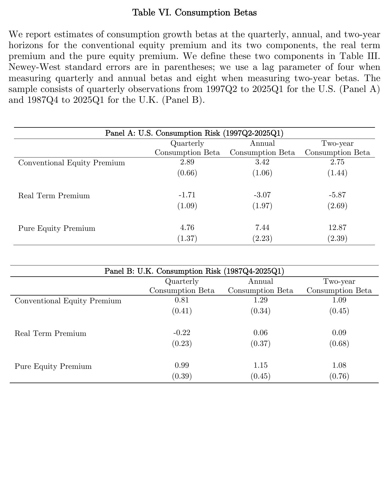
Having removed the bond leg, what is left looks much more like something a consumption-based model could price. The U.S. consumption beta rises from 2.89 for the conventional premium to 4.76 for the pure equity premium at a quarterly horizon, and from 2.75 to 12.87 at two years — the horizon strengthening that Daniel and Marshall documented. The real term premium’s own beta is negative at every horizon, which is to say the “safe” asset hedges consumption, as safe assets should.

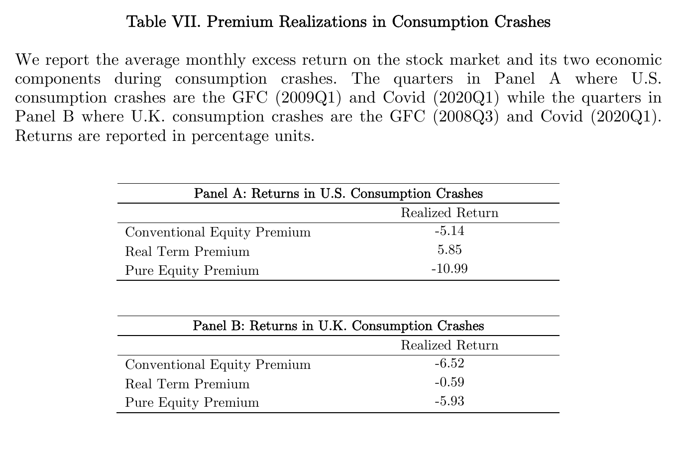
The crash evidence points the same way. Across the two consumption crashes in the U.S. sample — the financial crisis quarter and the Covid quarter — the conventional premium lost an average of 5.14% a month, while the levered real bond position made 5.85% and the pure equity leg lost 10.99%. The safe asset paid off exactly when consumption collapsed, which is what you would want it to do and what makes the equity part look properly risky.

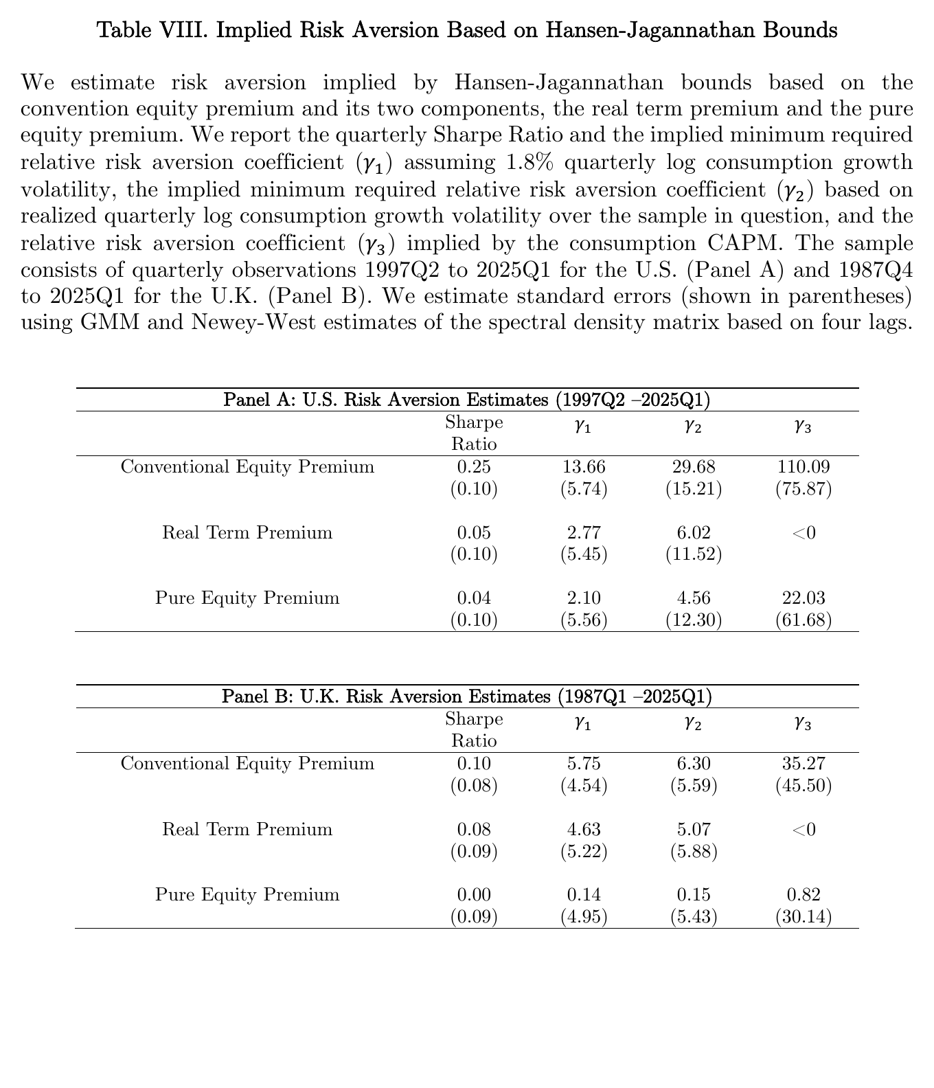
Feed that into the simplest possible Hansen–Jagannathan bound — time-separable power utility, minimum risk aversion equals Sharpe ratio over consumption-growth volatility — and the required risk aversion drops from about 13.7 to about 2.1 on the stockholder-consumption assumption, and from a frankly silly 110 to 22 on the consumption-CAPM calibration. Polk is honest about what that is worth: “certainly 22, as we go to the right, may not be that reasonable, but we’ve made substantial progress in going from 100 and to 22.” These are point-estimate statements; several of these gammas carry standard errors as large as themselves, and the table reports no tests of the differences. Note too what happens to the real term premium in the last column: it cannot be rationalized by any positive risk aversion, in either country, because its consumption beta is negative and its mean is positive.

Which is the actual result, and the paper says so: “to be honest, of course, we didn’t really solve the equity premium puzzle. What we’ve done is instead just sort of quarantined it safely within this real term premium bit.” The puzzle did not vanish. It moved into the leg nobody was looking at, where it is now much harder to explain, because the thing earning the premium is the thing that hedges you.

The problem with having only one bond market cycle

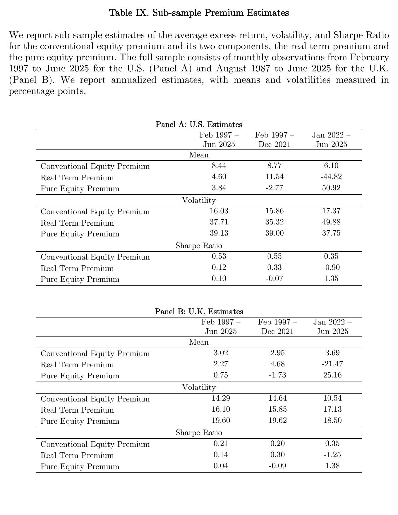
Inflation-indexed bonds are young: twenty-eight years of U.S. data, thirty-eight of U.K. All of it contains one great bull market in real duration and one violent unwind. How much does that matter? Run the sample to December 2021 and the real term premium averages 11.54% a year in the United States — more than the entire conventional equity premium — while pure dividend risk earned minus 2.77%. Add three and a half years and the bond leg returns −44.82% annualized over that stub, the pure equity premium 50.92%, and the full-sample signs flip back. The United Kingdom does the same thing. The paper notes drily that without frequent rebalancing “an investor invested in our (levered) real term premium series would have been liquidated by their broker.”

Polk is refreshingly direct about the authorial hazard: they started the project in early 2022, when the data said one thing, and “we don’t want to write papers that are going to change after just three years of data.”

The econometrics, which is the actual contribution

The honest response to “my estimate flips when I add three years” is not a robustness table, it is a better estimator. And the reason you need one is arithmetic. Lo’s standard error for a Sharpe ratio,

says that at the Sharpe ratios in play here — around 0.2 — you need roughly a century of annual data to distinguish the thing from zero. Nobody has a century of TIPS.

So the paper buys precision with an economic assumption instead of with data. Suppose the yield on a constant-ten-year-maturity inflation-indexed bond is strongly stationary. Then its monthly change has a population mean of exactly zero, and you can use that change as a control variate. Compare estimating a mean the usual way with estimating it as a regression intercept,

where $d(t)$ is the yield change. The equality is between population quantities; the estimators — the sample mean and the fitted intercept — are free to disagree in any finite sample, and the whole point is that they do. What the second equation removes is the part of the realized premium attributable to the fact that yields happened to trend one way over your particular twenty-eight years. In the paper’s words, it “asks the question what the premia would have been if the interest rates had not trended in either direction by chance.” Polk calls the setting “perhaps the near ideal real data use case,” and he has a case: the variance reduction is largest when the control variate explains a lot of the return and is itself very persistent, and real term premium realizations load on real-yield changes almost mechanically.

The constant-$\gamma$ requirement costs something, though, and it is worth being precise about what. Under the original recipe the leverage moves month to month, so the yield sensitivity does too. For this table the paper rebuilds all three series at a constant duration — fifty years in the United States, thirty in the United Kingdom — levering and delevering both legs. That is a different object, and it moves the U.K. answer before any control variate is applied: the U.K. real term premium sample mean falls from 2.27% to 0.47% and the pure equity premium rises from 0.75% to 2.83% on the re-leveraging alone. The right comparison is therefore constant-duration sample mean against control-variates intercept, not the earlier table against this one.

Done that way, the estimator delivers. In the U.S. sample the standard error on the real term premium falls from 6.39 to 2.71 and on the pure equity premium from 6.91 to 4.20, while the conventional premium’s barely moves at all — because the control variate explains only 2.6% of it, against 76.6% and 59.8% for the components. The method helps precisely and only where the control variate has something to explain, which is a nice property for an estimator to have. Stability improves too: across the truncated and full samples the sample-mean real term premium swings 12.21 to 4.52 while the intercept moves only 5.51 to 4.12.

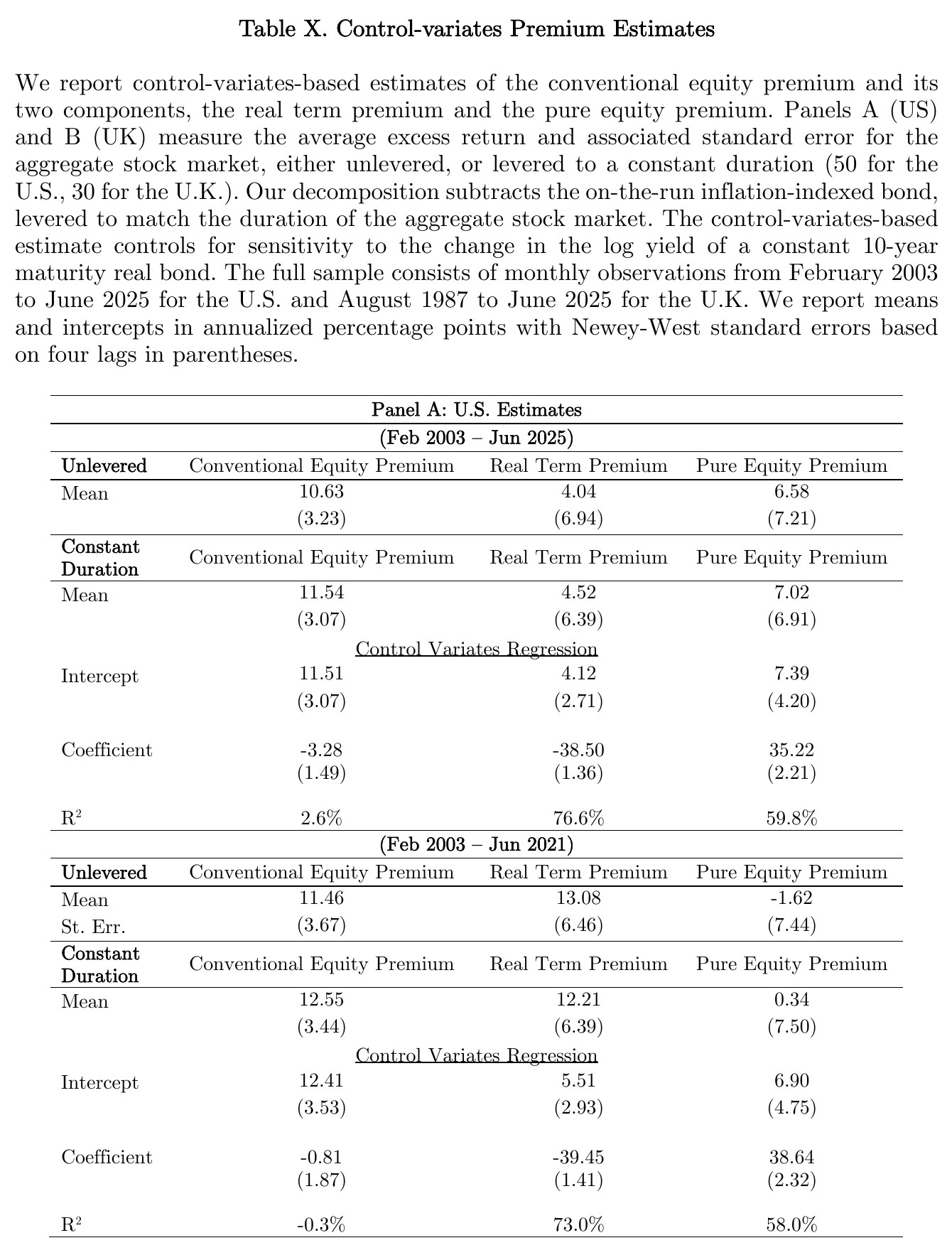
The headline numbers the paper is willing to put its name to come out of those intercepts: a mean real term premium of 4.12% in the United States and −0.44% in the United Kingdom, and a mean pure equity premium of 7.39% and 3.45%. Which, note, reverses the raw sample-mean story — the U.S. split becomes roughly two-thirds equity and one-third bond, and the entire meagre U.K. premium is assigned to dividend risk after all.

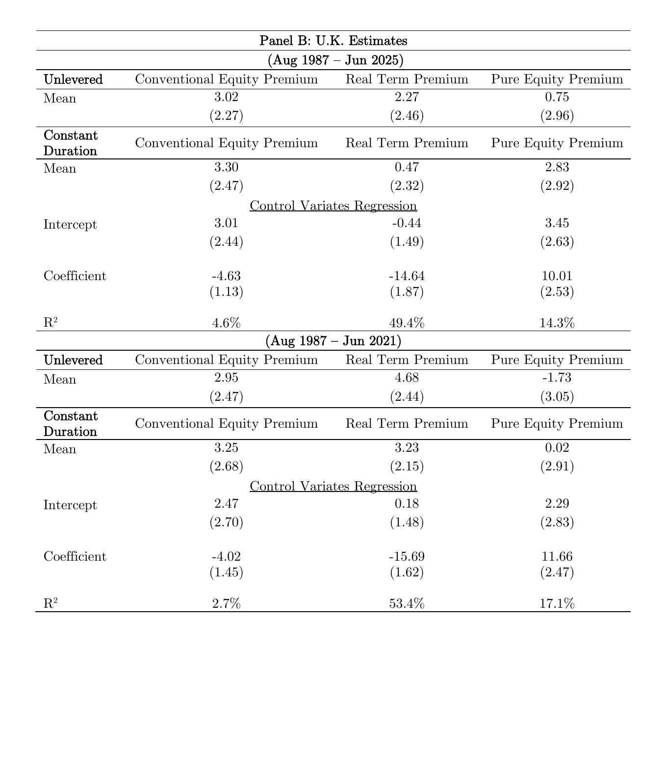
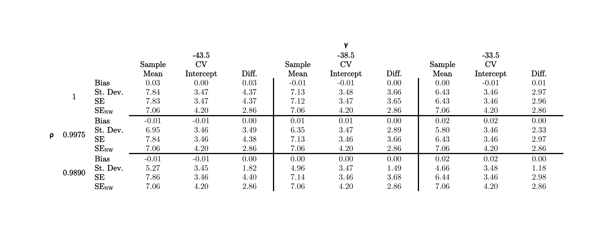
A Monte Carlo backs the intuition. Simulating 100,000 pseudo-samples of 269 months at the estimated loading, the intercept is essentially unbiased and its dispersion falls from 7.13 to 3.48 when the yield is a random walk, with the gain shrinking as the yield mean-reverts faster — exactly the predicted pattern. Two things a referee should notice in that grid. First, the random-walk case is nonstationary and the intercept is still unbiased, which locates the real failure mode precisely: what the estimator needs is zero-mean yield changes, not stationarity as such, so the danger is a systematic drift or a one-way shift in $r^*$, not persistence. Second, the reported Newey–West standard errors on the intercept (a median of 4.20) exceed its actual dispersion (about 3.47), meaning the paper is understating its own precision.

What a sharp referee would push on

(A note on sourcing: no discussant was assigned to this paper and the recording carries no questions, so what follows is not the room’s, it is the obvious reading.)

The −0.91 is partly built in. The pure equity premium is defined as the conventional premium minus the bond leg, and the bond leg dominates the variance of both, so a strongly negative correlation is close to arithmetic — and any measurement error in the bond leg is added to one component and subtracted from the other. The paper’s replies are real but partial: the results survive large changes in the scale parameter, the U.K. needs essentially no leverage at all, and the purged-residual correlation of −0.86 is genuinely hard to explain as pure construction. But no formal errors-in-variables bound is offered.

Then there is the single-cycle problem, which the paper concedes and answers with the estimator. That answer has a circularity of its own: the estimator’s validity rests on an assumption about the long-run behaviour of the very yield whose one-way regime shift is the thing you were worried about. It buys precision with an economic restriction, not with independent history.

Levering a 21-year TIPS by 2.8 is also not the same as owning a 55-year one. Convexity, the shape of the unobserved far end of the real curve, the actual financing cost, the liquidity and indexation and deflation-floor frictions of long linkers, and — the paper’s own example — the possibility of being margin-called all enter. The defence is a parallel-shift argument: 20-year and 30-year constant-maturity TIPS yields move so nearly together through the post-2021 selloff that “one must squint to tell the 20-year and 30-year TIPS yields apart.” Fair enough, but that series starts in February 2010, covering about 54% of the U.S. sample and leaving the first thirteen years untested.

A 55-year duration from the reciprocal of a dividend yield is a strong artefact of the buyback era, and the paper knows it: the same formula applied to the 1872–2000 average U.S. dividend yield gives 21.3 years. The alternative — using total payout including net repurchases — is discussed and asserted not to matter in aggregate, without a table. And one wrinkle is simply unresolved: the prose defines the control variate as a plain change in the constant-maturity yield, while the table notes call it the change in the log yield, with no transformation stated anywhere and real yields having gone negative in both countries during the sample. The paper is demonstrably aware of negative real yields — it floors them at a basis point in the duration formula for exactly that reason — so this reads as a notation question for the authors or the code, not as an error.

The leg nobody was looking at

The paper ends where it should, which is on the leg it moved the puzzle into. The real term premium has a positive mean, a negative consumption beta in both countries, a volatility exceeding that of the whole conventional equity premium, and a correlation of −0.91 with dividend risk. In other words it is an asset that pays you handsomely for holding the thing that protects you. What theory now has to produce, in the paper’s careful phrasing, is a shock that makes “the current value of a fixed real consumption stream decline while simultaneously either increasing future firm cash flows or reducing the expected future pure equity premium” — and it cannot be a cash-flow shock, because measured cash-flow news does not do it.

Polk put “safety” in scare quotes throughout the talk, and the paper asks the question directly: “Exactly what is the ‘safety’ of real bonds, anyway, if that safety requires a consistent and large risk premium?” Forty years of trying to explain why stocks pay so much, and it turns out that about half the mystery was about why bonds do.