Endogenous Technological Change Along the Demographic Transition

Write output per person in a Cobb-Douglas economy as the product of three things: technology Z, the capital-output ratio raised to α/(1−α), and the fraction of the population that works (eq. 1 in the paper). Population ageing is supposed to push on the last two: it lowers the employment share, and it raises the capital-output ratio, because people who expect to live longer save more. In calibrated life-cycle models the employment effect usually wins: Krueger and Ludwig (2007) and Ludwig, Schelkle and Vogel (2012) find cumulative declines in output per capita “on the order of 10 percent” over the twenty-first century (p. 1). In those models the first factor is an exogenous trend. Demography moves the machines and the workers; it never touches the ideas.

Markus Pettersson of Stockholm University, presenting his 27 May 2026 draft at the nber virtual workshop on the macroeconomic effects of population aging, points out that this is a slightly odd thing to assume. The extra saving has to go somewhere. In the textbook it all goes into machines; in the actual economy some of it goes into R&D, and what that buys is ideas, which are nonrival. A machine raises productivity only through capital per effective worker. An idea raises everyone’s productivity at once. So if ageing raises saving and some of the saving buys ideas, the technology term moves too, and it can move more per dollar than the capital term does. The headline is that it moves enough to flip the sign. In his model the us demographic transition raises output per capita by a cumulative 27.5 percent between 1950 and 2100. The same model with technology made exogenous gives −12.2 percent, which is roughly the Krueger–Ludwig number (pp. 27–28).

He was candid about where this started. “My prior was that tfp would sort of switch the … impact of the demographic change into a positive rather than a net negative. And because of that, I sort of deliberately had a very conservative … way of modeling things when whenever I had a choice” (02:23:48). That is an unusual thing to say out loud, and a reasonable way to handle a prior: every free modelling choice goes against you, and you see whether the result survives.

The motivating fact is a binscatter. Across oecd countries from 1970 to 2020, one more year of life expectancy at age 20 goes with a saving rate 0.70 percentage points higher and an intellectual-property investment rate 0.20 points higher, after partialling out country effects, relative prices and dependency ratios (Fig. 1, pp. 1–2). The calibrated model produces 0.57 and 0.15 without targeting them. The paper calls the oecd slopes descriptive rather than causal (p. 21), which is the right amount of weight.

The model: a life-cycle economy that saves into patents

The model bolts two standard frameworks together, and Pettersson says plainly that the bolting is the contribution: “the sort of core contribution here is the merger of these two types of modeling strands … I’m sort of deliberately being … pretty standard within each of these blocks” (02:22:30). The household block is Auerbach–Kotlikoff (1987), with income risk, endogenous hours, an absorbing retirement choice, warm-glow bequests, and a pay-as-you-go pension whose replacement rate is fixed while the payroll tax balances the budget. The production block is Romer’s (1990) expanding varieties with Jones’s (1995) semi-endogenous R&D technology. The only exogenous input is age-specific fertility, mortality and migration. The economy is closed, “a standard and conservative benchmark” (p. 7), on the argument that ageing is global and ideas cross borders, so openness should strengthen the R&D channel.

The asset market is the one piece of plumbing that carries the argument. Household wealth is capital plus equity in patent-holding intermediate firms, A_t = K_t + P_zt z_t (eq. 30, p. 13), and no-arbitrage sets the return on a patent, which is its monopoly dividend plus capital gain net of obsolescence, equal to the return on a machine (eq. 22, p. 11). So the household sector is, among other things, a venture fund: retirement savings buy claims on firms that do not yet exist. When an ageing population wants to hold more wealth, both asset classes get funded. The R&D block and technology are:

In eqs. 19, 21 and 24 of the paper, Q_t is R&D spending in units of the final good, z_t the measure of varieties, λ the duplication (“stepping on toes”) elasticity, ϕ the knowledge spillover, δ_z the rate at which intermediate firms become obsolete, and Z_t the labour-augmenting tfp the varieties add up to, with 1/ρ the markup. λ = 0.75 is imposed. ϕ = −0.068 is backed out from us tfp growth of 1.11 percent a year and ipp investment growth of 5.97 percent (pp. 17–18; Table 3, p. 16). That is mildly negative, “consistent with this … ideas getting harder to find paper” (02:34:26), a reference to Bloom et al. (2020), and it implies a scale elasticity of tfp γ_Z = 0.22, mid-range of Jones’s (2002) estimates (p. 18).

The paper’s three-generation toy model shows where the results come from. Its steady-state tfp is

where sr is the saving rate, ρ̄ the share of saving allocated to capital (so 1 − ρ̄ goes to R&D), and L_t^γ the scale term (eq. 4, p. 5). The bracket is what the paper calls R&D intensity, the R&D twin of capital deepening: save more, and ideas per unit of scale go up. The second factor is pure nonrivalry: a larger population permanently raises the level of technology. In the toy model a temporary fertility boom leaves the intensities unchanged in the long run but raises Z permanently, through L alone (Table 2, p. 7).

The device that makes the exercise work is the one the room returned to most. In semi-endogenous growth, steady-state per-capita growth is proportional to population growth n. Model ageing as a permanent fall in n and, as Pettersson put it, “you mechanically impose that … it’s going to lower gdp growth” (02:18:27). He argues that post-war us demography is mostly two transitory events, the baby boom and rising survival after 50, and survival gains after the childbearing years leave long-run n alone. He therefore gives the initial 1900 steady state and the terminal steady state the same n = 0, set through a migration shifter; the un’s 2100 rates rolled forward give roughly zero anyway (pp. 14–15). The economy learns the entire demographic path in 1901 and has perfect foresight thereafter; moments are sampled over 1901–1949, so everything after 1950 is a prediction rather than a fit (pp. 14, 19). With the same trend at both ends, every result is a temporary growth effect that leaves a permanent level effect: “temporary in the sense that you know it might go on for 100 years but still temporary” (02:31:26).

The numbers, and a small bookkeeping problem

Anyway, here is what the transition does. The paper’s growth accounting splits per-capita growth into tfp, capital intensity, employment rate, hours and efficiency per hour (Table 4, p. 25):

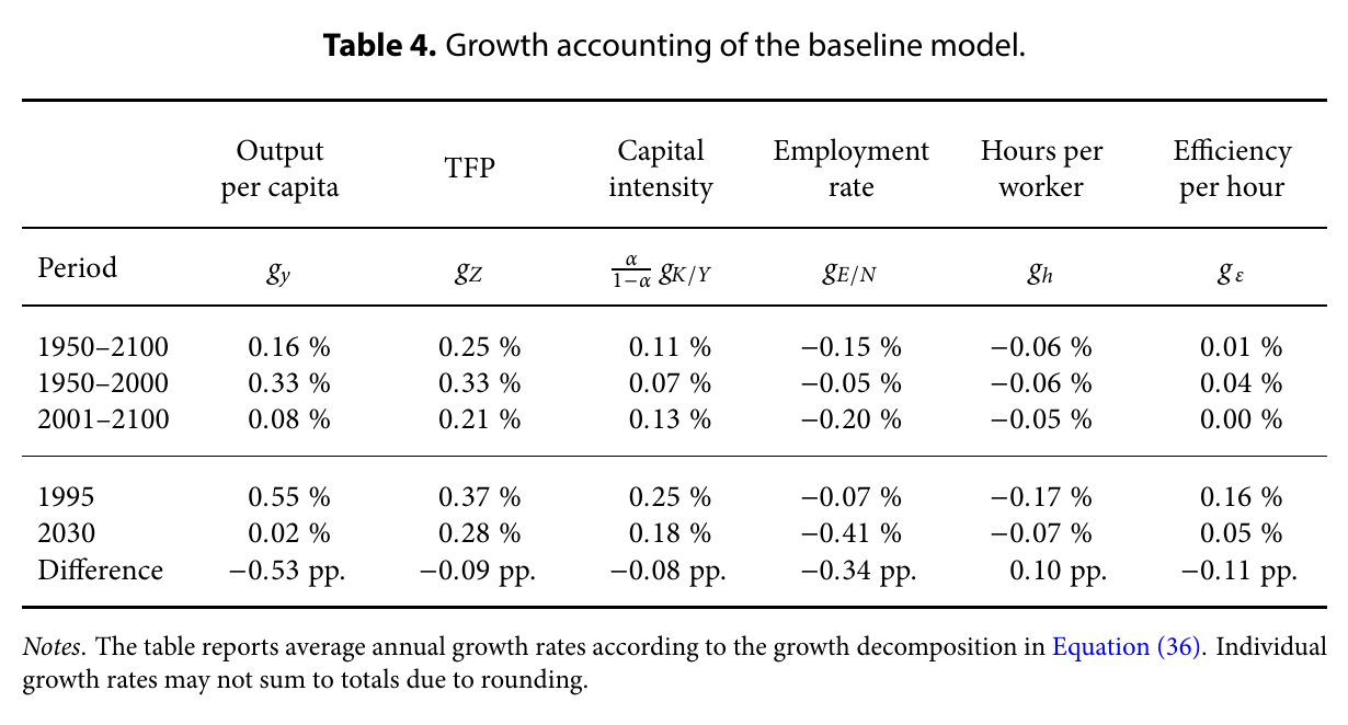
Over 1950–2100 the transition adds 0.16 percentage points a year to per-capita growth; over 1950–2000 it adds 0.33, and over 2001–2100 just 0.08. The talk rounded the second to “around 0.3” (02:19:44). Cumulated, that is the 27.5 percent level gain (p. 26). The employment rate is the drag throughout, −0.15 a year overall and −0.20 in the twenty-first century, because the retirement age barely moves while life expectancy does (p. 25). tfp more than pays for it.

Against us per-capita growth of “approximately 2 percent per year”, the paper says “over 15 percent” of post-war growth is due to transitory demography, comparable to Fernald and Jones’s (2014) roughly 20 percent for education (p. 24). The abstract says “15 to 20 percent”, and in the talk the denominator became 1.82 percent, which is how 0.3 turns into “roughly 15 to 20%” (02:20:18). “Over 15 percent” is the version that survives the paper’s own arithmetic.

The ratio of tfp to capital deepening drifts more. The abstract says technology’s contribution “triples that of capital deepening”; the introduction says “three to four times” (p. 3); page 24 says “about two and a half times” over the full period and “about five times” over the twentieth century. The table says 0.25 against 0.11 for 1950–2100, about 2.3 times; 0.33 against 0.07 for 1950–2000, about 4.7 times; and 0.21 against 0.13 for 2001–2100, only about 1.6 times. “Triples” appears in no row of Table 4, and the twenty-first-century ratio is the one that matters for anyone reading this in 2026. tfp is still the largest positive term in every row, so the result survives; the adjectives should be brought in line with the table.

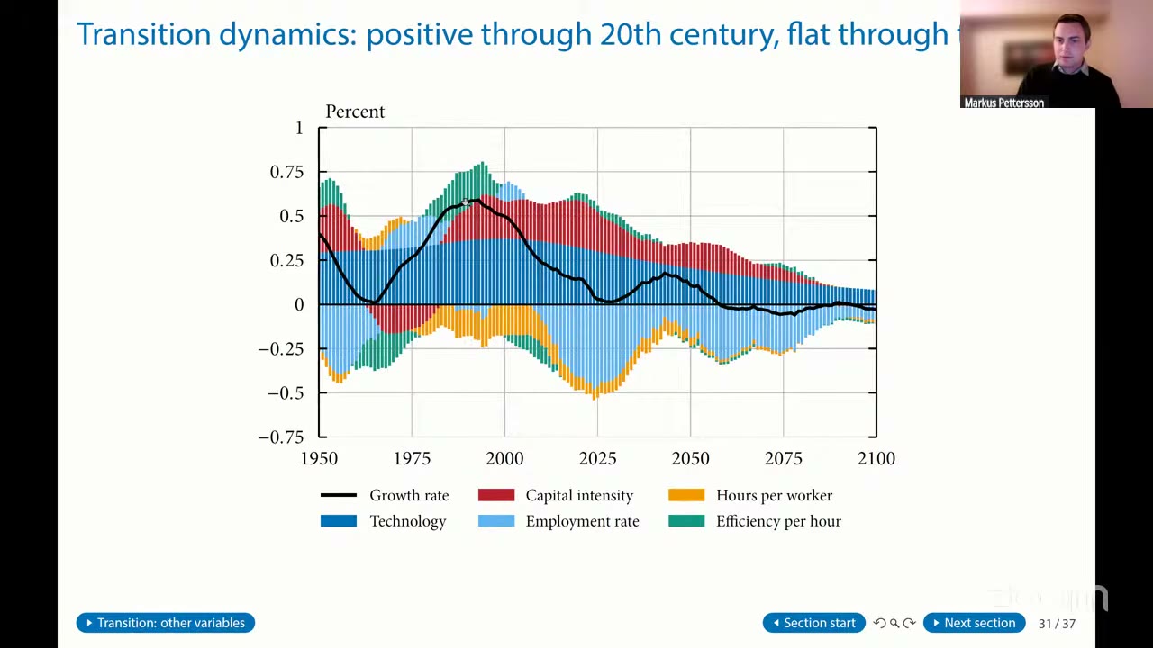
The time path is the more interesting object. The growth effect peaks in 1995 at 0.55 points and has collapsed to 0.02 by 2030, a drop of 0.53 points, 0.34 of which (65 percent) comes from the employment rate as the baby boom retires; tfp, capital intensity and efficiency each lose about 0.1 (Table 4 and p. 25). That looks like the secular-stagnation story, and Pettersson says so, but he reads it differently. The trend is zero by construction, so this is not ageing doing damage; it is the above-trend growth the boomers generated in their prime years running out: “it’s effectively the good times sort of fading out” (02:37:05). The reversion would occur even without rising life expectancy (p. 25). From about 2030 the effect hovers around zero.

Why technology moves so much when so little saving goes to it

tfp dominates, but not because most saving goes to R&D. Capital investment exceeds R&D investment by a factor of 4 through most of the transition (fn. 22, p. 22). The answer is in a steady-state decomposition that mirrors eq. 4. Between the 1900 and terminal steady states output per capita rises 45 percent, tfp 72 percent, the capital-intensity term 17 percent, and the employment rate falls 22 percent (Fig. 7, p. 23). And the 72 percent splits as an 18 percent rise in R&D intensity times a 47 percent rise in scale (p. 23; backup slide at 02:45:25). The behavioural channel lifts R&D intensity by about as much as capital intensity, 18 percent against 17. What makes tfp different is the second factor, which capital does not have.

It is worth being precise about that second factor. Scale is steady-state employment raised to γ_Z = 0.22, so a 47 percent scale effect requires terminal-steady-state employment of about 5.8 times its 1900 level (my arithmetic, not the paper’s; with population as the scaling variable the scale effect is 55 percent, fn. 24, p. 23). That is not ageing. That is several times as many Americans at the end as at the start, all using the same ideas. The paper doesn’t hide this, and it is exactly what nonrivalry means, but it changes how you read the headline: in the steady-state comparison, the largest piece of “the demographic transition raises output” is “the population got much bigger”.

The counterfactuals say the same thing from another angle. Chop off the baby-boom hump in fertility and remove the post-1950 gain in adult life expectancy, one at a time and together, and the 27.5 percent decomposes into 8.2 points from the baby boom, 3.0 from falling mortality after 50, and 14.7 from everything else, with a negligible interaction (Fig. 10, pp. 26–27; 02:39:01, where “the increase in old age mortality” is a slip of the tongue for the decline). “Everything else” is the non-stationary 1950 age structure plus the remaining demographic changes that keep raising the population and so feed scale (p. 27). The recognisably ageing piece, longer lives after 50, is 3 of the 27.5 points. It is positive, which is the interesting part: here living longer pays for itself in output per head, narrowly.

Shut off the ideas and you get the old answer back

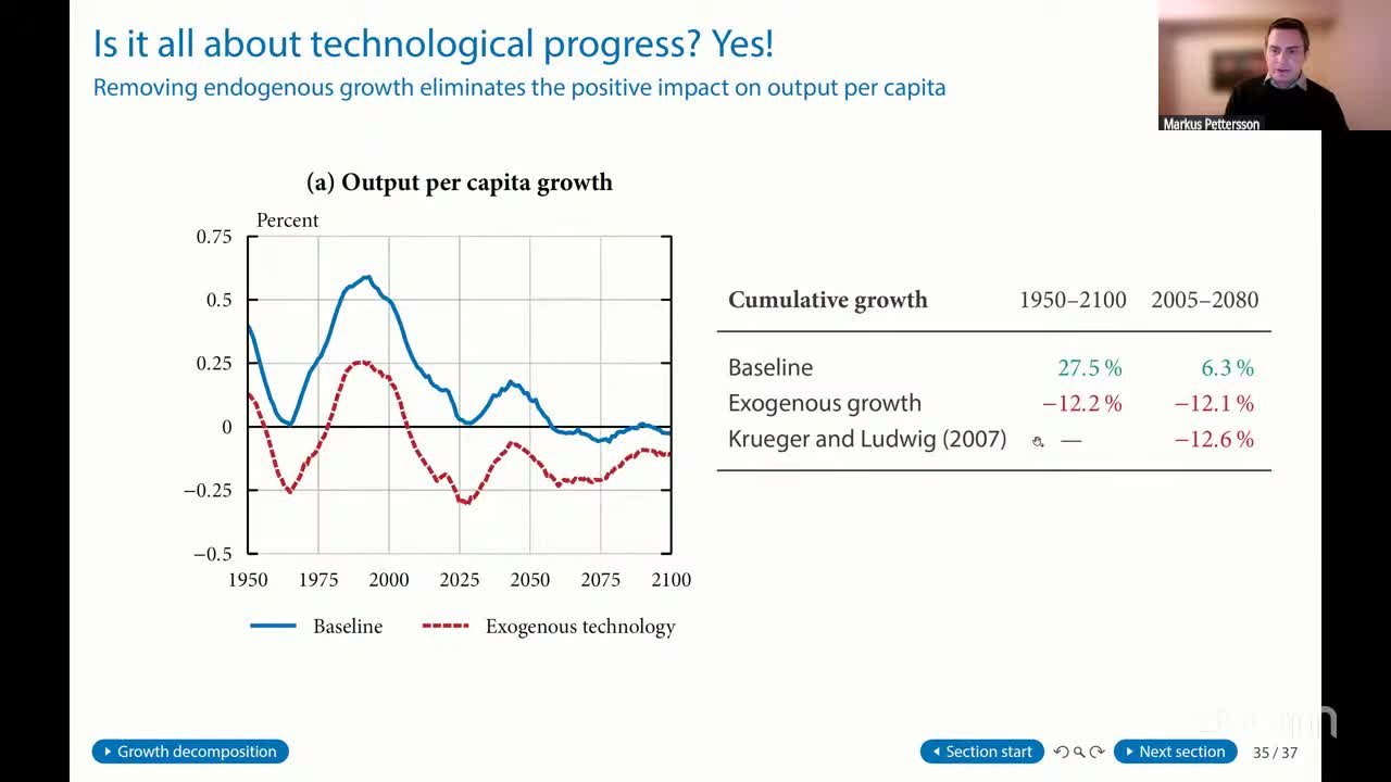
The cleanest exhibit removes the mechanism. The model nests an exogenous-growth olg model: set ρ = 1, so intermediates are perfect substitutes, profits vanish, and the patent price and R&D go to zero; set δ_z = 0, so the measure of firms stays constant; recalibrate β, ψ, Ω_A and δ_k to hit the same targets (p. 27). Growth then runs 0.1 to 0.4 points below baseline throughout. The cumulative change over 1950–2100 goes from +27.5 percent to −12.2 percent, and over 2005–2080 from +6.3 to −12.1 percent, against Krueger and Ludwig’s −12.6 percent for the same window (pp. 27–28; 02:40:30). The gap between the two runs is almost entirely tfp; capital intensity, the employment rate and efficiency are virtually unchanged, with a small offsetting rise in hours (Fig. 11b, p. 28).

This exhibit does real work: it rules out the worry that a rich new olg model differs from the old answer for reasons unrelated to R&D. Switch the ideas channel off and it lands within half a point of the canonical estimate, so the tfp channel is the only thing standing between this paper and Krueger–Ludwig. Nor is it fragile to the obvious knob. With weaker spillovers (ϕ = −1.4, γ_y = 0.07) or stronger ones (ϕ = 0.4, γ_y = 0.36), 1950–2100 average growth moves by about 0.1 to 0.15 points; labour as the R&D input changes essentially nothing; only the most pessimistic setting turns the twenty-first century negative, at about −0.02 percent a year (pp. 28–29).

What the room pushed on

There was no discussant; questions came from the floor, and the names below come from auto-captions, so they are hedged. Most circled the n = 0 device.

The first came mid-talk, from a participant who appears to be the “Yui” (presumably Yuhei Miyauchi) called on later: is population constant in the long run? Yes. The follow-up: Jones’s (2022) “Empty Planet” paper shows innovation stagnating when population growth is negative, so is the optimism here just the assumption that it isn’t? Pettersson said he was “not arguing against that paper at all”: survival gains after childbearing age shouldn’t move steady-state n, so they must be analysed outside the steady state, and in that sense the paper is “very much a complement” to Jones (02:33:17). Later the same questioner came back with the sharper version: what if the long run is a balanced growth path with a shrinking population? He conceded it: “I haven’t run the model with negative … population growth. … I could do that” (02:55:45). The normalisation does separate a transitional effect from a change in trend, but it also makes the reassurance conditional on the trend being the benign one.

“Adrian” (presumably Auclert, one of the organisers) pressed the same point from the other side: isn’t innovation here driven by the current population growth rate rather than the age structure, and wouldn’t results then be sensitive to the un’s low-fertility variant, where growth reverses by 2100? Pettersson’s answer was that tfp depends on both, and he pulled up the backup slide with the +72 = +18 × +47 decomposition, R&D intensity being “effectively the result of changes in household behavior, the saving rate and so on” (02:45:28). That answers the age-structure half. The fertility-variant half went unanswered, and given how much rides on scale it is the run I would most like to see.

“Larry” (presumably Laurence Kotlikoff, whose name is on the household block) brought four points (02:46:11): the young are the innovators; nobody in 1950 anticipated Nixon’s double indexing of Social Security or Medicare, surprises that would move forward-looking saving; capital flows; and bequests are involuntary. The answers: R&D uses output made by workers with a hump-shaped productivity profile, a labour-input variant gives the same results, and evidence on innovators’ age is thin; with a fixed replacement rate and payroll taxes adjusting under perfect foresight, pensions are set up in what the paper calls “the most growth-pessimistic arrangement” (p. 12), though policy surprises are not modelled; a closed economy is conservative; and warm glow dampens the saving response to longevity, another deliberately conservative choice (02:49:08–02:51:22).

“Diego” asked the policy question (02:52:14): standing in 2026, will demography lower growth relative to the past decade? The answer was that the demographic effect “remained around zero … from around 2030 up until the end of the century”, so neither boost nor drag (02:55:17). True from 2030 on, though Table 4’s 0.53-point fall from 1995 to 2030 means the model does imply lower growth than at the late-1990s peak; most of that fall has happened by 2026, and what remains is its tail.

“Luis” (presumably Luis Teles Morais) asked about the return on capital, given Auclert and coauthors’ (2021) falling returns. It falls from around 4.2 percent in 1950 to around 2.2 percent at century’s end, about a point of it after 2000 (02:56:58); those numbers are talk-only, as the paper plots the path without stating them.

More ideas, mostly from more people

So: take the model that says ageing costs you 12 percent, add that some saving buys ideas and ideas are nonrival, and get +27.5 percent. That is a well-built result, and the exogenous-technology run makes it hard to argue the new machinery is doing anything other than what it claims. But look at where the 27.5 comes from. About 3 points are from people living longer after 50. About 8 are from the baby boom, a fertility event. The largest piece is everything else, much of it the population getting bigger, and the tfp decomposition agrees, with scale at 47 percent against 18 for R&D intensity. The paper finds that “these findings leave little reason to worry about current demographic change” (p. 3). The mechanism that delivers that reassurance is, mostly, more people. The paper assumes the population stops growing rather than starts shrinking, and the room’s most persistent question was what happens if it does.

References