Technological Revolutions and Stock Prices

Ľuboš Pástor and Pietro Veronesi, American Economic Review 99(4) (September 2009), pp. 1451–1483. Published version, with the Technical Appendix; no recorded talk.

Pástor and Veronesi’s paper is about the rise and fall in the stock prices of firms using a new technology, which everyone calls a bubble and almost everyone blames on irrationality. Shiller (2000) and Perez (2002) are the citations for the irrational view, and the paper’s epigraph is The Economist in September 2000 noting that technological revolutions and financial bubbles “seem to go hand in hand”. The paper offers a different account, with no irrationality in it, and the account rests on a fairly simple point. A new technology is risky in two different ways at two different times. When it is a curiosity run by a few firms, its risk is idiosyncratic, and idiosyncratic uncertainty about growth makes a stock more valuable. When it is about to be installed across the whole economy, the same uncertainty becomes everyone’s risk, which means it is priced, which means discount rates go up. A technology that turns out to be good enough to adopt has to make that trip from one regime to the other, and the stock prices of the firms using it rise on the way out and fall on the way in. Seen from afterwards, the round trip looks exactly like a bubble.

That last sentence is doing a lot of work, and much of the paper is about being careful with it. The “bubble” is visible only ex post, conditional on knowing that the revolution happened. Nobody in the model expects prices to fall, and across all the histories the model generates, realized returns equal expected returns. The hump appears only when you select the histories that ended in adoption, which is what economic historians do whenever they write about railroads or the Internet.

The mechanism: a laboratory economy, and a risk that changes owners

You are a representative agent with power utility over terminal wealth, risk aversion $\gamma > 1$, and a horizon $T$. You own one big economy, the “old economy”, whose capital $B_t$ compounds at a productivity rate $\rho_t$ that mean-reverts to $\bar\rho$. Everything is reinvested, and at $T$ you consume what has accumulated. At date $t^*$ someone invents a new technology. If you adopt it, the long-run mean of your productivity becomes $\bar\rho + \psi$. You do not know $\psi$; your prior is normal and centred on zero, with standard deviation $\hat\sigma_{t^*}$. Adoption is irreversible and costs a fraction $\kappa$ of your capital.

You would not adopt immediately. With a prior centred on zero, adopting loads a symmetric gamble on the productivity of your entire wealth, with no expected gain to pay for it, which a risk-averse agent refuses even when conversion is free (Proposition 1). What you do instead is set up a laboratory. You run the new technology in a “new economy” of capital $B^N_t$, infinitesimally small next to $B_t$, whose productivity $\rho^N_t$ mean-reverts to $\bar\rho + \psi$. Because it is infinitesimal, it costs nothing and has no effect on your wealth. It exists purely to generate data: by watching $\rho^N_t$ against $\rho_t$ you learn about $\psi$, and your posterior mean $\hat\psi_t$ is a martingale while your posterior variance $\hat\sigma^2_t$ falls deterministically. Experimenting is optimal because it is a free option (Proposition 3), and the option is worth more the more uncertain the technology is. (The paper adds that if experimenting were costly, or you had to choose among several technologies, you would pick the most uncertain ones to try, other things equal. In the model as solved, the one technology is always tried for free.)

At a decision date $t^{**}$ you adopt if what you have learned clears a hurdle, eq. 8 in the paper:

where $\tau^{**} = T - t^{**}$ is the time left after adoption and $\varphi$ is the speed of mean reversion in productivity. The first term pays for the conversion cost and the second for the uncertainty you are about to load onto your whole wealth, so the hurdle is always positive. You adopt without knowing the true $\psi$; you just think it is good enough. The paper fixes $t^{**}$ to get closed forms, and later lets you choose it optimally, like exercising an American option, with similar dynamics. A “technological revolution” is defined as the stretch from $t^*$ to $t^{**}$ in a history that ends in adoption.

Now price things. There are two stocks, one paying the old economy’s terminal capital and one paying the new economy’s, and the stochastic discount factor is your marginal utility of terminal wealth. Let $p_t$ be the probability, as of $t$, that adoption will happen at $t^{**}$. At invention it is small; in the baseline calibration it is about 0.02. The whole paper turns on eq. 12, the dynamics of the discount factor:

where $\tilde Z_0$ is the shock to old-economy productivity, $\tilde Z_1$ is the learning shock (news about $\psi$, filtered out of the new economy’s productivity, whose own noise is $\sigma_{N,1}$), and $S_{\pi,t}$ is how much marginal utility cares about that news. When $p_t$ is zero, $S_{\pi,t}$ is zero. News about $\psi$ is news about a laboratory, your wealth does not depend on it, and so it is not priced. As $p_t$ goes to one, $S_{\pi,t}$ rises to $\gamma A_2(\tau^{**})$. The same news is now news about the productivity of everything you own. Nothing about the technology has changed; what has changed is who is going to be exposed to it. That is the paper’s sense of uncertainty moving “from idiosyncratic to systematic”, and it happens before adoption, through anticipation, which is why prices can fall before anything is physically installed.

So an upward revision in $\hat\psi_t$ does two things to the new economy’s market-to-book ratio. It raises expected cash flows, and the new economy feels this immediately, because it already runs the technology. It also raises $p_t$, which makes $\psi$-risk more systematic and raises discount rates; this effect grows with $p_t$ and also bites harder on the new economy, whose returns load directly on $\psi$-news. For small $p_t$ the cash-flow effect provably wins (Proposition 7); the authors compare it to a deep out-of-the-money option, whose delta is small. Near $t^{**}$, the paper says, the discount-rate effect “usually dominates”. And in a history that ends in adoption, $\hat\psi_t$ has to drift upward between $t^*$ and $t^{**}$, because that is what it means to clear the hurdle. Feed a rising $\hat\psi_t$ through an effect that is positive early and usually negative late, and you get a hump.

The one surprising thing

The sharpest statement of this is Corollary 2, and it is the thing to take away from the paper. Hold your beliefs fixed and compare the new economy’s valuation at $t^{**}$ in the two knife-edge cases where $\hat\psi_{t^{**}}$ sits just above the hurdle (adopted) or just below it (not adopted), eqs. 15 and 16:

with $A_1$ and $A_2$ evaluated at $\tau^{**}$ and $\overline C_0$ a deterministic term given in the Technical Appendix. The posterior variance enters with coefficient $+\tfrac12 A_2^2$ when the uncertainty is idiosyncratic: this is the convexity result of Pástor and Veronesi (2003), where uncertainty about a firm’s growth raises expected compounded cash flows and therefore its value. Once adopted, the coefficient is $\tfrac12 A_2^2(1-2\gamma)$, which is negative for any $\gamma > 1/2$. The same uncertainty that used to raise the valuation now lowers it. Adoption gives the new economy nothing (it already uses the technology) and takes something away: its risk becomes the economy’s risk.

The old economy’s value can fall at $t^{**}$ too, if adoption happens with $\hat\psi$ close to the hurdle. And you adopt anyway. You own both stocks, adoption can lower the market value of everything you own, and it still raises your expected utility, because stock prices are marginal utilities, not utility. Adoption puts you in a world of higher expected wealth and higher discount rates, which is better for you and worse for your portfolio’s mark-to-market. Read uncharitably, this is the paper saying that the market is right to crash on good news; read correctly, it is saying the market crashes on good news about the economy because that news is bad news about risk.

The calibration and the simulated revolution

Table 1 is the calibration: $\bar\rho = 0.1217$, $\varphi = 0.3551$ and all three productivity volatilities at 0.07, “close to” the authors’ own 2006 estimates for the dynamics of profitability. The prior standard deviation of $\psi$ is 0.04, conversion costs 10 percent, the revolution lasts eight years, the horizon is 30 years, and $\gamma = 4$. None of this is estimated in this paper, and it should be read as an illustration of the mechanism, not a fit. The authors simulate 50,000 histories and split them by whether adoption happens; in the plots invention is at year 1 and the decision at year 9. Since $p_{t^*} \approx 0.02$, the revolution-conditioned averages describe a rare subset of histories.

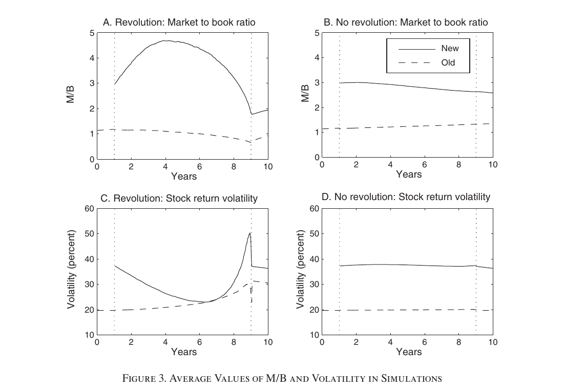
Figure 3 is the hump. Conditional on a revolution, the new economy’s average market-to-book goes from about 3 at invention to about 4.7 around year 4 and down to about 1.8 at $t^{**}$ (my reading of the graph; the text gives only the decline). On the average path the fall from peak to trough lasts five years and is 2.9 units of M/B; in 10 percent of revolutions it takes less than 2.6 years, and in 5 percent the drop exceeds 7.8. The old economy’s M/B drifts down gently; for it, the discount-rate effect “generally outweighs” the cash-flow effect from the start. The new economy’s volatility is U-shaped: high near $t^*$, where the cash-flow effect dominates; low in the middle, where the two effects roughly cancel; high again near $t^{**}$. The spike exactly at $t^{**}$ comes from paths that land right on the hurdle, and it disappears when $t^{**}$ is chosen optimally, so it is not a robust prediction. Without a revolution, nothing much happens.

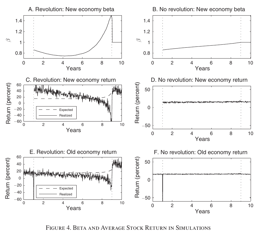
Figure 4 holds what is, to my mind, the paper’s best prediction: the new economy’s beta. Good news about $\psi$ generally lowers the old economy’s value, and early on it raises the new economy’s, so the two move apart and beta falls. Once the discount-rate effect takes over, good news lowers both, so they move together and beta rises. In the simulations beta doubles in the second half of the revolution, from 0.75 to 1.5. The bottom panels make the selection point explicit: in revolutions, realized returns run first above and then far below expected returns, and “across all 50,000 simulations, average realized returns are equal to average expected returns.” The rise and fall, in the authors’ phrase, are “observable ex post but not predictable ex ante.” The sensitivity analysis (Figure 5) says the hump survives $\gamma = 3$ and $\kappa = 0$, so conversion costs are not what drives it. It gets bigger with more prior uncertainty ($\hat\sigma_{t^*} = 0.08$) and with faster adoption (six years instead of eight), which is the abstract’s claim that bubbles are largest for “technologies characterized by high uncertainty and fast adoption”. (The text says the horizon would also be varied; no figure varies $T$.) With optimal adoption timing the hump is “slightly weaker”, averaged over histories where the optimal $t^{**}$ falls between years 8 and 10.

The evidence: the Internet

The empirical sections are structured as a comparison of shapes, and the authors are careful to frame the result as consistent with a joint hypothesis: that the model holds, and that the technology was adopted on a large scale at a particular date. For the Internet the new economy is nasdaq and the old economy is nyse/amex, 1992–2005, using daily crsp index returns. To set up the comparison, they rerun the model with a six-year revolution, on the grounds that the Internet spread fast. In that run (Figure 7) beta falls from 0.9 to 0.7, rises to 1.65 at $t^{**}$, and then falls back to 1. Old-economy volatility doubles to 38 percent, new-economy volatility exceeds 65 percent, and new-economy market value quintuples and then halves. Old-economy productivity starts rising only after adoption.

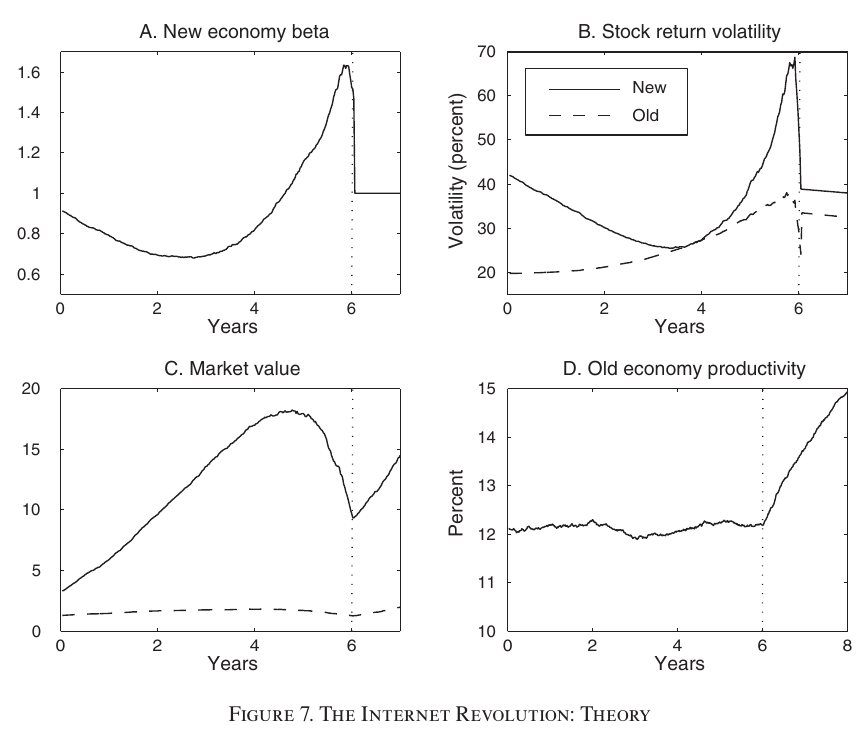
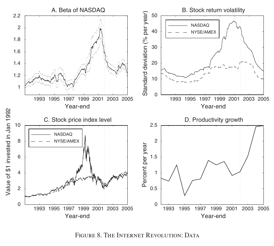
Figure 8 is the data. nasdaq’s beta on nyse/amex (rolling 500 trading days, with two-standard-error bands) dips slightly from about 1.2, then doubles from 1.0 to 2.0 between 1997 and mid-2002. nasdaq volatility goes from 17 percent in 1992 to 11 percent in 1995 to 47 percent at the start of 2002; nyse/amex goes from 13 to 8 to 21 percent by the end of 2002. nasdaq quadruples between 1996 and March 2000 and is back at its 1996 level by October 2002, while nyse/amex has a much smaller rise and fall. Multifactor productivity growth (bls, three-year average) is about 1 percent a year through the 1990s and then 1.5 percent in 2003 and 2.5 percent in 2004 and 2005. The model plots productivity levels and the data shows growth rates, a substitution the paper defends in a footnote. The dotted line marks October 2002, and the paper’s conclusion is that the evidence is “consistent with the joint hypothesis that our model holds, and that the Internet technology was adopted on a large scale by 2002.”

The interesting thing here is not that nasdaq went up and came down, which nobody needed a model for. It is the beta. A story in which investors got carried away and then sobered up has no particular reason to make nasdaq more correlated with the rest of the market at the bottom. A story in which Internet risk was becoming the economy’s risk predicts exactly that. The conclusion says this directly: predictions involving the new economy’s beta “are unlikely to follow from behavioral models, in which there is typically no role for systematic risk.”

The evidence: railroads, 1830–1861

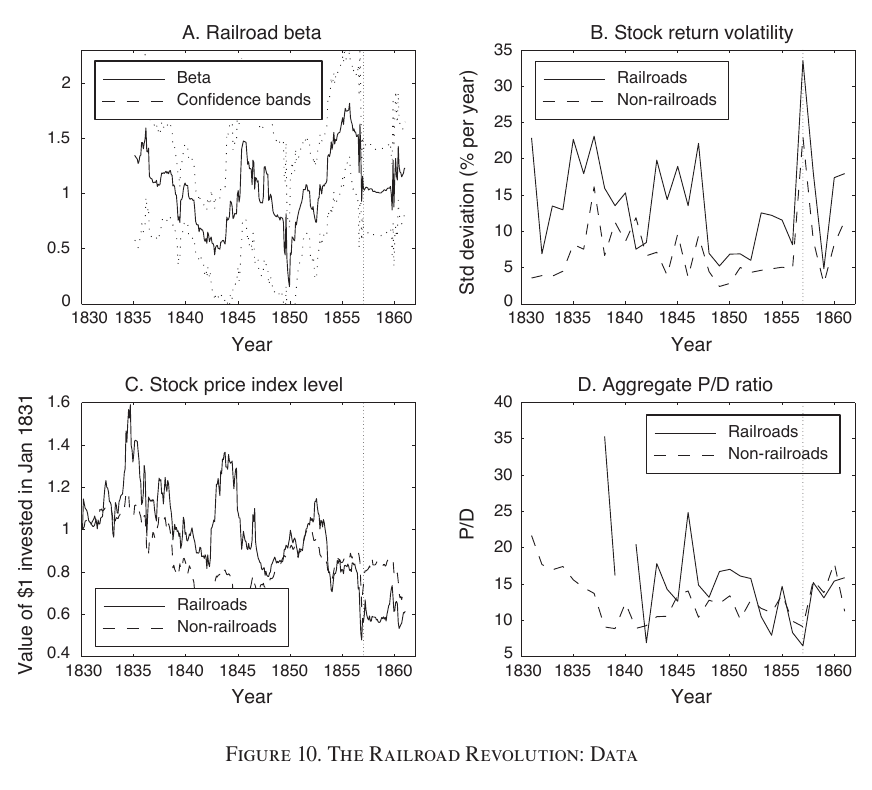
The railroads are the “out-of-sample” test, and the data are much thinner. The prices are monthly nyse prices from the Goetzmann, Ibbotson and Peng (2001) database, with railroads picked out by name. The indices are price-weighted capital gains, not total returns, because dividends are annual and spotty. Before 1848 no month has more than five railroad stocks with valid returns, so gaps of up to three months are filled by linear interpolation (the authors say the results without it are noisier but lead to “the same basic conclusions”). Beta, from 36-month rolling regressions with wide bands, rises from about 0.2 in 1850 to about 1.8 in 1856 and falls to about 1.0 right after 1857. Railroad volatility exceeds non-railroad volatility in every year except 1841, and in 1857 it jumps to 33.5 percent, against 23.1 percent for non-railroads. From June 1853 to October 1857 the railroad index falls 58.3 percent and the non-railroad index 33.9 percent. The railroad price-dividend ratio goes from 24.9 in 1846 to 15.8 in 1852 to 6.5 in 1857; the non-railroad ratio goes from 14.0 to 12.8 to 9.1. Mileage went from 9,021 in 1850 to 30,626 in 1860, and in 1856 the first railroad bridge crossed the Mississippi. The paper concludes, again as a joint hypothesis, that this looks like large-scale adoption “around 1857”.

The obvious problem is that 1857 is also the year of the Panic of 1857: the embezzlement at Ohio Life in August, gold lost at sea in September, and bank failures by October. The authors list these themselves and reply with Mishkin (1991), who dates the financial disturbance months before the October panic and finds the spread between low- and high-quality corporate bond yields higher in 1857–1859 than at any later time before the 1930s. High credit spreads mean high risk premia, and the authors call Mishkin’s remark that falling stock prices “might be linked to the general rise in interest rates” “precisely our story.” That is fair as far as it goes. A rise in discount rates is what their model predicts, but it is also what a banking panic produces, and the spread does not tell you which one you are looking at.

Weak points, my own reading (no discussant exists)

The adoption date is not measured independently of the evidence. In both episodes, $t^{**}$ is placed where the beta peaks and prices bottom out, and the match between model and data is then read off the same series. The authors are honest that this is a joint hypothesis, and they bring in outside markers (the post-2002 productivity acceleration; Cochrane (1979) and Craig and Weiss (1993) on productivity growth around the Civil War). But nothing here is a test against a model in which there was no technological revolution and something else raised systematic risk in 2001–2002 or 1857. With 36 monthly observations per railroad beta, the bands are wide enough to fit a lot of shapes.

The model also has no investment boom, and the paper says so in its conclusion. The new technology is tried on a negligible scale, so the model “fails to predict the large amount of investment that often accompanies technological revolutions”, and the unused fibre of the 1990s is outside it. The authors allow that irrationality may contribute both to that overinvestment and to the prices; their claim is that rising beta is hard to get without systematic risk, not that behavioural biases play no role. Their productivity-versus-profitability concern, that gains might go to workers rather than shareholders, is handled in the Technical Appendix with a labor-income extension. There the mechanism survives because discount rates depend on total wealth, though the bubble is weaker at the same parameters.

Finally, there is the representative agent. The planner adopts on one date across the whole economy, which is an odd picture of how railroads or websites spread. The paper shows that competitive, value-maximizing firms with network externalities can replicate the planner’s adoption threshold and prices, but only with the externality set exactly as the appendix requires, and the result that no firm adopts at $t^*$ is a limiting one, valid for small enough $p_{t^*}$. Gradual diffusion through heterogeneous conversion costs is suggested but not solved. The decentralized version does make one point nicely: each adopting firm ignores that its adoption raises systematic risk for everyone else, which is a negative externality in discount rates.

None of this dents the main contribution, which is an idea rather than a measurement. “Bubble” usually means prices that were wrong, and this paper produces the same picture with prices that were right at every date, given what investors knew. In the model, the stocks that crashed were priced correctly throughout, and the crash came from the technology working well enough to be adopted.

References