Financial intermediation, resource allocation, and macroeconomic interdependence

Galip Kemal Ozhan (University of St Andrews), “Financial intermediation, resource allocation, and macroeconomic interdependence,” Journal of Monetary Economics 115 (2020), pp. 265–278. The paper is the first chapter of his dissertation. No recorded talk was found, so this is read from the paper alone: no discussant, no Q&A, and the online appendix it cites for the banker’s problem was not available to us. Version used: the published article.

In 2007:QIV only about 45% of the deposits in Spanish financial institutions belonged to Spanish residents (the paper’s footnote 1, citing Santos 2017). The rest was, more or less, the rest of the euro area lending to Spain through Spanish banks. Those banks then lent disproportionately to builders, developers and mortgage borrowers, not to the firms making things Spain could sell abroad. You know how the decade ended. The consensus version, which Ozhan quotes from Baldwin and Giavazzi in his conclusion, is that “capital flows tended to feed non-tradable sectors in the periphery of the Eurozone, and when the investors lost trust in deficit nations, the effects of a sudden-stop were amplified due to the predominance of bank financing.” The paper’s project is a two-country model in which that sentence falls out of a banker’s first-order conditions.

Here is the principle. You are a Gertler–Karadi banker. You have some net worth, you raise deposits, and once you have raised them you can walk off with a fraction of what you bought. Depositors know this, so they fund you only up to the point where staying in business is worth more to you than running. The shadow price of that incentive constraint shows up in every spread you charge. Ozhan’s twist is that the stealable fraction depends on the asset. A claim on the non-traded sector (construction, services, housing, and the securitised paper wrapped around them) is harder for depositors to monitor than a claim on a traded-goods firm, so more of it can go missing. In equilibrium the spread on each asset is the constraint’s multiplier times that asset’s divertability.

That is a one-factor pricing model. The factor is how tight the bank’s constraint is, and each asset’s loading on it is how easy the asset is to steal. The opaque asset is the high-beta asset, and high-beta assets are the ones that rally hardest when the factor moves. When foreign creditors grow more confident in Spanish banks, the multiplier falls, every lending spread falls with it, and the non-traded spread falls about three times as far in basis points because its loading is about three times as large. The opacity that made construction credit expensive in the steady state is exactly what makes it the big winner in the boom. It is also, symmetrically, what makes it the big loser when the confidence leaves.

Anyway, that is what the paper calls the banking channel. There is a second, trade channel that needs no heterogeneity across bank assets at all, plus a policy section in which a common central bank buys non-traded claims or lends against them. The evidence is a quarter-by-quarter fit to Spain, a pair of counterfactual calibrations, and two policy experiments.

The model

Two countries of equal size, Home (read Spain) and Foreign (read the core), symmetric except for the shock. The model is real, with no nominal rigidities, and is solved by log-linearising around the non-stochastic steady state. Households consume a CES bundle of traded and non-traded goods, the traded part being a home-biased bundle of Home and Foreign varieties, and they supply sector-specific labour. They save only in one-period riskless bank deposits, at home or, for a small quadratic cost, abroad. Deposits are the only asset that crosses the border, so international markets are incomplete. Goods producers in each sector finance all of next period’s capital by selling claims to domestic banks, and banks monitor firms perfectly, so the entire friction sits between the banker and her depositors. Capital producers face convex adjustment costs, which is what makes asset prices move. Bankers survive each period with probability $\gamma$, so they cannot simply grow out of the constraint.

The constraint is the paper’s eq. (16):

Here $V_t(N_t(j))$ is banker $j$’s franchise value given net worth $N_t(j)$, $\lambda_T$ and $\lambda_{NT}$ are the stealable shares of traded and non-traded assets, $Q_{i,t}S_{i,t}(j)$ is the value of her claims on sector $i$, $B^*_{t+1}(j)$ is what she has raised from Foreign households, and $\iota_t$ governs how much of the foreign-funded part is off limits.

That last symbol deserves a moment. The paper calls $\iota_t$ “the relative degree of friction applying to Foreign deposits,” and interprets its movements as swings in international confidence in the Home financial sector. Look at where it sits, though: it subtracts foreign-funded assets from the stealable base. So a rise in $\iota_t$ is a fall in friction, and the boom in this paper is $\iota_t$ going up. It is a confidence index wearing the name of a friction. (Notice too that $\iota_tB^*_{t+1}$ comes off both brackets, so a unit of foreign money relaxes the constraint by $(\lambda_T+\lambda_{NT})\iota_t$ whatever it happens to fund. We come back to this below.)

The first-order conditions (18) and (19) set the discounted spread on traded and non-traded lending over the Home deposit rate equal to $\mu_t\lambda_T$ and $\mu_t\lambda_{NT}$, where $\mu_t$ is the multiplier on (16). Eq. (20) prices the two kinds of deposit:

where $\beta$ is the discount factor, $\Lambda_{t,t+1}$ the household marginal-utility ratio, $\Omega_{t+1}=1-\gamma+\gamma\nu_{t+1}$ the banker’s shadow value of a unit of net worth, $R^H$ the rate Home banks pay Home savers and $R^F$ the rate they pay Foreign ones.

So Home banks pay foreigners more than they pay their own savers, because foreign money loosens the constraint and is worth a premium. In the paper’s words, “a unit of Foreign deposit allows Home intermediaries to expand assets by greater amount and intermediaries are willing to pay a premium for this advantage.” The best funding a bank can have, in this model, is foreign money, whose value to the bank is precisely the thing the shock later takes away.

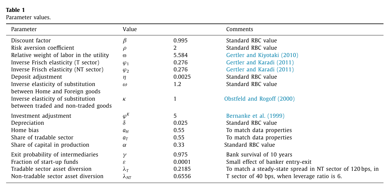
The calibration is standard except for the banking block. $\lambda_T=0.2185$ and $\lambda_{NT}=0.6556$ are chosen jointly to deliver steady-state lending spreads of 40 bps in the traded sector and 120 bps in the non-traded one at a leverage ratio of 6, which is where the “about three times” comes from. The empirical case for a higher $\lambda_{NT}$ is that the 2003–2015 average mortgage rate exceeded the rate on loans to non-financial corporations in Spain, and that securitisation of real-estate assets, negligible before 2000 and about 30% of total bank credit by 2008 on the cited estimates, made bank obligations more opaque. The steady-state $\iota$ is set so that the Foreign–Home real deposit spread is 158 bps, to match “the difference between the 1993–1999 and 1999–2015 average of the short-term real interest rate spread between Spain and Germany”; the implied value of $\iota$ itself is not reported. (Table 1 labels $\gamma$ an “exit probability,” but at 0.975 it is the survival probability, as the text says.)

The boom

The shock is $\iota_t=\iota e^{\psi_t}$ with $\psi_t$ an AR(1) at persistence 0.99, “because joining to the Eurozone was seen as an irreversible event.” Ozhan feeds in a sequence of same-signed shocks every quarter from 1999:QIV to 2008:QI, 33 of them, each “allowing for a 50 percent reduction in the frictional costs of cross-border deposits” (we could not reconstruct from the text exactly what 50% per quarter cumulates to). In period 33 a single counteracting shock takes $\iota_t$ back to its 1999:QIV value. That is the sudden stop.

Follow it through. A higher $\iota_t$ shrinks the stealable base, so $\mu_t$ falls and the leverage limit loosens for any given net worth. The lending spreads have nothing pushing back: they are $\mu_t$ times a constant, so they all fall, the non-traded one most. Non-traded firms borrow more, bank portfolios tilt toward them, and the non-traded share of output rises. The deposit spread in (20) is the one place with a tug-of-war, since a lower $\mu_t$ shrinks it and a higher $\iota_t$ widens it. The paper’s footnote 14 is candid that the sign depends on which wins. In the baseline $\iota_t$ wins, $R^F$ rises relative to $R^H$, Home banks pull in Foreign deposits, and Home runs “a persistent and climbing current account deficit.”

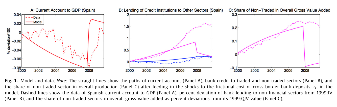
Fig. 1 sets this against Spain, and the boom looks right. Reading by eye, and all of these are approximate: the model’s current account slides roughly linearly to about −0.08 on the chart’s scale by 2008, against a Spanish series that drifts to about −0.06 and dips to around −0.08. Model credit to the non-traded sector is up about 83% by 2007:QIV while traded credit is up about 20%, the same divergence as in the data, although Spanish non-traded credit grew further still (about 145% by 2008). The non-traded share of value added rises about 21% in the model against about 25% in the data. Ozhan’s own summary is that the model “reasonably captures” the current account and the credit divergence during the boom. (The credit comparison is not quite like for like: the data are lending per GDP, the model series are $Q_TS_T$ and $Q_{NT}S_{NT}$.)

The bust is another matter. At the stop the model’s current account jumps to about +0.03 within a quarter, whereas Spain’s recovered gradually, reaching about +0.01 by 2009. Model non-traded credit falls from about +0.83 to about +0.38 and then +0.22, and the non-traded share drops to about −0.09, below its pre-euro level, while in the data the share stays up around +0.21 to +0.24. The paper says as much, that the non-traded variables fall “in a more pronounced manner vis-à-vis to the data,” and offers the missing ECB as “one of the reasons.”

The trade channel, and a sign that flips

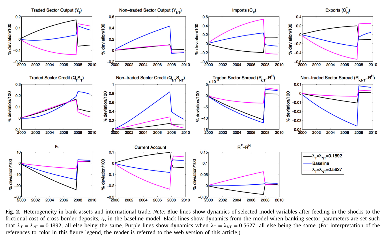
To pull the channels apart, Ozhan turns the heterogeneity off. The “high lambda” economy sets $\lambda_T=\lambda_{NT}=0.5627$ (120 bps steady-state spreads in both sectors) and the “low lambda” one sets both to 0.1892 (20 bps each). With equal $\lambda$s the two lending spreads move one for one, so any tilt toward non-traded credit has to come from the demand side. It does, through the trade channel: cheaper foreign funding lowers the Home real interest rate, asset and consumption prices rise, Home goods get expensive, households switch to imports, exports fall, the traded sector shrinks and wants less credit. Capital inflows produce an intra-national imbalance next to the international one without any help from bank opacity. In the high-lambda economy this is the whole story, and it is a big one: on the chart the current account reaches roughly −0.23, imports rise by roughly 55% and exports fall by about as much, and non-traded credit still outgrows traded credit. In the baseline, credit growth to the non-traded sector exceeds the ratio $\lambda_{NT}/\lambda_T$, which Ozhan reads as the two channels adding up: “Banking channel (i.e., λNT > λT) reinforces trade channel.”

The low-lambda economy is the more interesting one. When bankers can steal little, $\mu_t$ falls much further (about −23 on the chart, against about −14 in the baseline), and its fall swamps the $\iota_t$ term in (20). The Foreign–Home deposit spread goes negative (about −0.04 on the chart), Home’s relative interest rate rises, Home goods get cheaper, exports rise, imports fall, and Home runs a current-account surplus of roughly +0.09 with a growing traded sector. The same “foreigners trust our banks more” shock runs the trade channel backwards. So the Spanish pattern, the deficit and the construction boom, is in this model a high-agency-cost outcome and not a generic consequence of financial integration. To a macro reader that may be the paper’s most surprising result, and it is also a sign that the level of $\lambda$ is carrying a lot of weight.

One discrepancy with the text. The paper says the sudden stop produces “a one time hike in the traded output” in the baseline only, “not present in the other two versions as the credit spreads move equally.” Fig. 2 shows high-lambda traded output jumping as well, from about −0.14 to about +0.135, a bigger jump than the baseline’s; only the low-lambda economy has no spike. Our reading of the panels, not the author’s: what is baseline-only is the credit rebalancing, since traded credit rises at the stop only in the baseline. The high-lambda output jump comes with exports leaping from about −0.55 to about +0.24, the trade channel reversing. The stated reason explains the credit move, not the whole output spike.

The central bank arrives

Section 4 adds a common central bank, notionally at the zero lower bound, that targets only the non-traded sector from 2008:QI, with a policy innovation of size 5, “implying an absolute deviation of 500 from zero” (footnote 26 compares this with response coefficients of 100 in Gertler–Karadi and 400 in Dedola et al.). Under asset purchases it holds a share of non-traded claims itself, financed by interest-bearing reserves raised equally from banks in both countries, and banks can divert those reserves at $\lambda_{ECB}=\lambda_T/2$, assumed “w.l.o.g.” Under liquidity facilities it lends to banks at rate $R_m$ against non-traded claims and reserves, and whatever is pledged can no longer be diverted. Either way the policy is a swap: the bank gives up its most stealable asset and gets back something depositors find easy to watch.

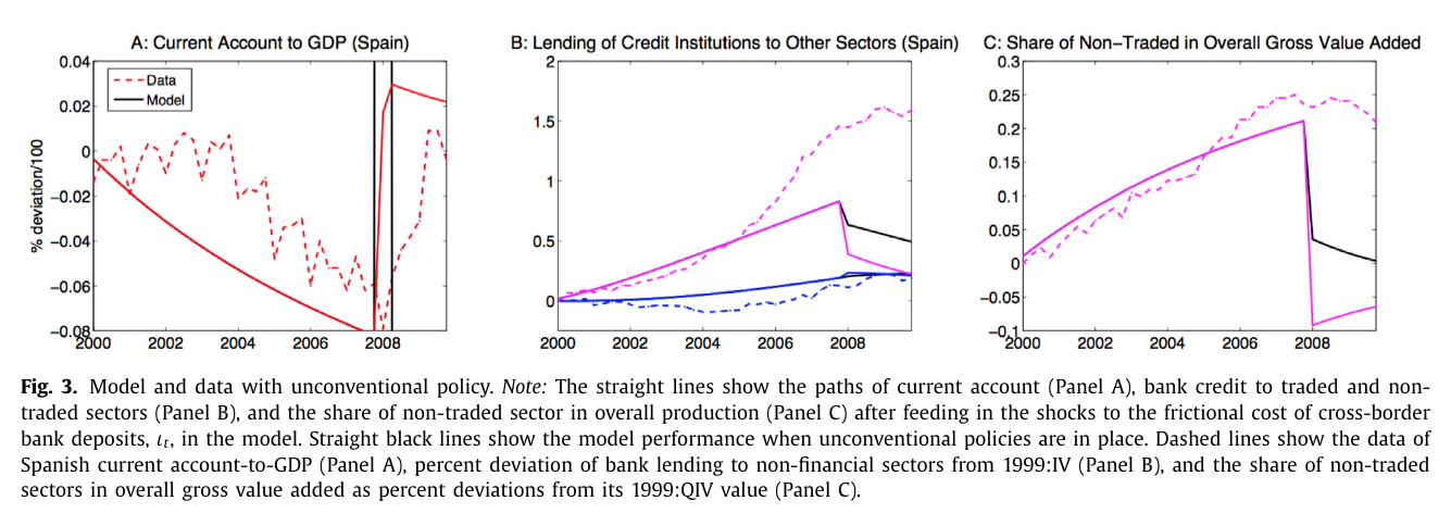
Fig. 3 runs the two together, “the combination of central bank asset purchase program and liquidity facilities.” Policy is strong enough to push non-traded credit spreads negative. By eye, non-traded credit falls from about +0.83 only to about +0.63, and to about +0.5 by end-2009, against about +0.22 without policy. The non-traded share settles near zero rather than about −0.09. The central bank is channelling funds from Foreign to Home, so private outflows are “partially replaced by public capital inflows,” which is a tidy description of the euro area’s post-2008 plumbing. The one panel where you would most like to see that is the current account, and it shows only vertical spikes at 2008; the paper calls it “uninformative vis-à-vis to the data under UMP.” Even with policy, the lending collapse remains more severe than in the data, which Ozhan attributes to the Spanish regulatory measures of 2008–2010 left out of the model.

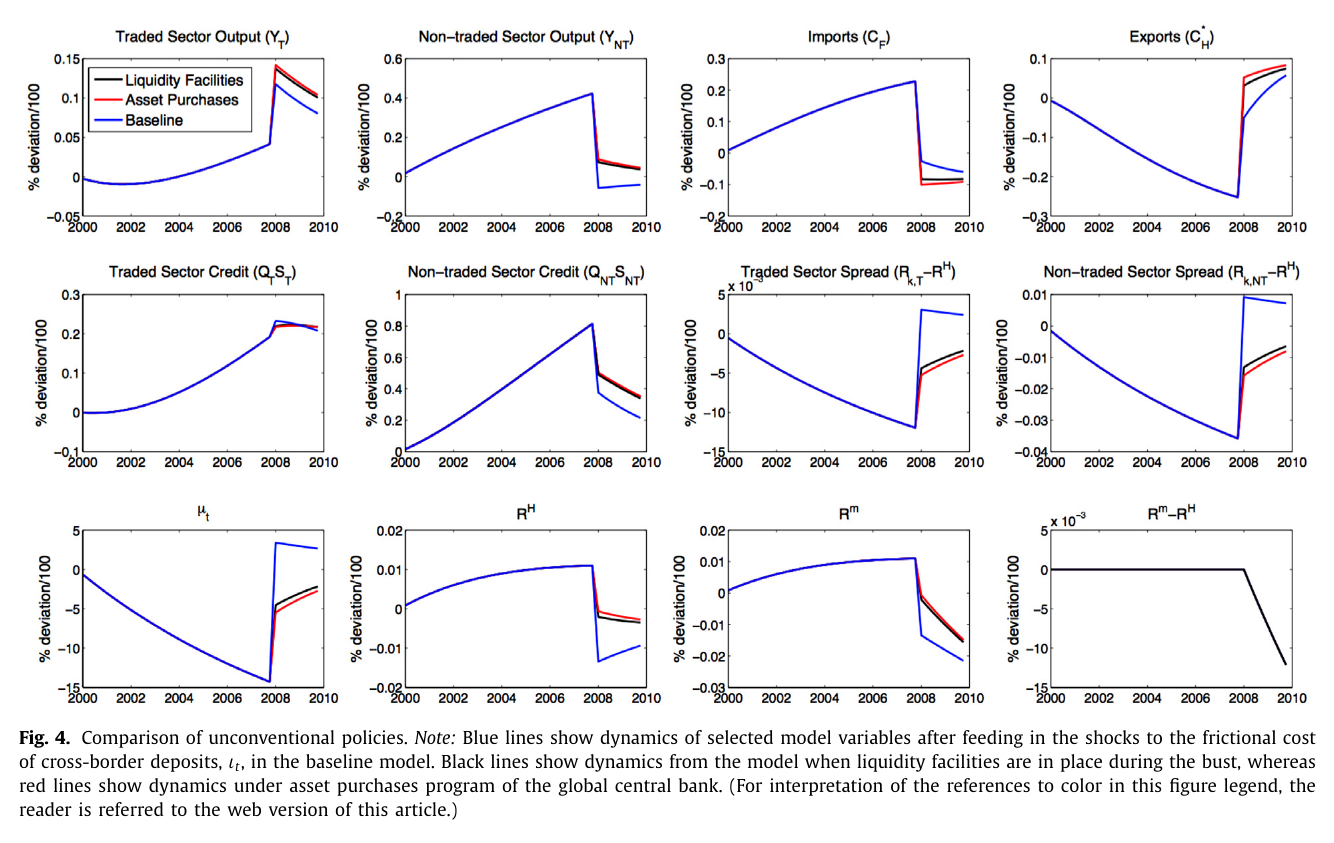
Fig. 4 runs them separately, and asset purchases come out “slightly better.” The theory said they shouldn’t. With no friction between banks and firms, extra funding routed through banks ought to be allocated efficiently, so liquidity facilities should win. They lose because of the size of the program. The facility rate ends up below the deposit rate, $R^m-R^H$ falling to roughly −12×10⁻³ on the chart by 2010, so central-bank money crowds private deposits off bank balance sheets. Ozhan names this plainly as a violation of Bagehot’s rule that liquidity should be lent “at a penalty rate.” The model built a lender of last resort that ignored Lombard Street and then ranked it second.

Objections (ours; there is no discussant)

First, one shock does all the work. The decade is 33 consecutive same-signed innovations at persistence 0.99 and then one reversal; footnote 21 grants that the size and persistence “contribute to the quantitative fit,” while insisting the qualitative features survive a milder process. Because the solution is log-linear, each quarter’s shock is a surprise and nothing endogenous produces the stop. The boom fit is therefore partly by construction, and the bust, the nearest thing to an out-of-sample test, misses badly on the non-traded share (a like-for-like comparison) and on the speed of the current-account swing, roughly 0.11 on the chart scale inside a quarter against Spain’s gradual adjustment. Second, the heterogeneity that drives the banking channel is a calibrated wedge. $\lambda_{NT}/\lambda_T\approx3$ is backed out of 120 versus 40 bps, and a positive mortgage-minus-corporate rate gap also reflects collateral, maturity, risk and fees. The securitisation story arguably cuts the other way, since securitised claims are easier to sell and pledge. Foreign deposits relax both sector brackets in (16) whatever they fund, with no stated microfoundation. The 158 bps target is a pre-versus-post-1999 change in the Spain–Germany spread used as a steady-state level. And Fig. 2 shows that the sign of the current-account response depends on the level of $\lambda$. Third, a first-order solution is being asked to handle a constraint that is being blown wide open. The baseline multiplier moves by about −14 in the chart’s “% deviation/100” units, non-traded credit rises about 80%, and under policy lending spreads go negative. A linearisation around a binding steady state cannot say whether the constraint stops binding, and negative spreads are the obvious warning sign. The zero lower bound is asserted in a real model rather than modelled. Relatedly, with perfect bank monitoring of firms there is no sense in which the non-traded borrowing is a misallocation (the paper says so), and welfare is never computed.

The swap

Strip the ECB names off Section 4 and what remains is a single trade. The bank’s problem, all along, was that its most profitable boom asset was also the one its depositors could least watch. The central bank takes that asset off its hands and gives it back reserves, stealable at half the traded rate. So the cure for opacity, in this model, is a counterparty that depositors find easy to monitor and that is, at this size, willing to be the cheapest money on the balance sheet. That is a fair description of a central bank, and some explanation of why, in 2008, every bank wanted to deal with one.