A Macroeconomic Model of the Cross-Section of Currencies

Aleksei Oskolkov and Diego Perez, presented by Oskolkov at the nber International Finance and Macroeconomics Program Meeting, 23 October 2026; discussant Charles Engel. This note uses the draft of July 17, 2026.

In 2008 the Australian dollar fell 39% against the us dollar, the Hungarian forint 25% and the Thai baht 15%. If you do international finance you have a tidy description of that: a couple of global factors, country-specific loadings, a nice $R^2$. If you do international macro you have a tidy story mapping shocks into an exchange rate, usually one exchange rate. The first camp can tell you which currencies move together and not why. The second can tell you why and not which.

Anyway, Oskolkov and Perez want to derive the factor regression from a macro model, so that each factor has shocks inside it and each loading is a country trait. The traits they pick are commodity exposure and dollar assets. They are candid about the selection: those are the two things the empirical loadings correlate with, so those are the two things they built in.

The model

Start with what a currency is here, because it is not money. There is no money. There is one tradable good, priced at one everywhere, and a local non-tradable, and “currency $i$” means the local consumption basket, whose price is $Q_{it}=(P^N_{it})^\alpha$. So the baht-dollar rate is, in effect, the price of a Bangkok haircut over the price of a Boston haircut. Haircuts cannot leave the country. Anything that puts more tradable spending in your household’s hands therefore bids up your non-tradable price and appreciates your currency, and every channel in the paper is a claim about who gets tradable spending in which state.

Now the two traits, both permanent and exogenous. The first is $e_i$: a global tradable shock $z$ lifts everyone by $e_i z$, so commodity countries get the bigger windfall, spend more and appreciate more. The second is the dollar stock. Each country has a manager (reserves, but Oskolkov wants you to think of pension funds and insurers too) following an imposed rule: when the broad dollar is strong, sell a little and rebate the capital gain to households. The percentage is common, so the absolute rebate scales with the stock, and more rebate means more tradable spending and a smaller depreciation. This is a long-dollar hedge whose payoff gets spent on haircuts. Answering what seems to have been a question about this (the room’s questions are off-mic), Oskolkov called the rule a stand-in and said an optimising problem might deliver something similar. That problem is not solved.

The wrinkle is that the hedge pays only on a relative basis. All that dollar demand has to be intermediated, and it comes back to everyone as inflows, so what matters is $m_i-m$. Insurance that every neighbour also bought is worth nothing to you.

The intermediary is the only balance sheet in both markets. Households trade only their own local bond; the one global intermediary has no capital, issues dollar bonds to meet reserve demand and places the proceeds in local bonds, tilted by expected returns and risk, with a quadratic penalty for straying from a uniform portfolio. Its sdf is the household-average sdf with extra weight $\Gamma_t=\Gamma(1+\gamma_t)$ on the stochastic part. Two risks survive into that sdf: low global tradable output, and low us non-tradable output. The second is priced only if $\rho>1$, and it survives the averaging only because the us is a mass point counted equal to the whole rest of the world. Together they make bad states strong-dollar states.

So who is risky? High-$e_i$ currencies are, and low-dollar currencies are, and the picture is lopsided on the safe side. Low $e_i$ is an outright hedge against global output risk. High $m_i$ only shrinks exposure to us output risk, which stays positive for most countries and flips sign only around $m_i\approx3.2$. A currency’s net riskiness depends on the pair, and only the dollar is safe by construction. Then $\gamma$ arrives. It moves no one’s aggregate consumption and carries no price of risk. It just reshuffles capital from risky countries to safe ones.

Take a first-order solution around the risky steady state, assume $e_u=e$ and uncorrelated $e_i$ and $m_i$, send $\chi\to\infty$ with $M_i/\sqrt{\chi}\to m_i$, and (Proposition 2 with eq. 10) the panel collapses to

Here $\Delta s_i$ is depreciation against the dollar, $z$, $x_u$ and $x_i$ are the global tradable, us non-tradable and local non-tradable shocks, $\gamma$ is the risk-aversion shock, $e_H$ and $e_L$ are mean exposures above and below the median, $\tau$ is the reserve elasticity, $\alpha$ the non-tradable weight, $\rho$ the inverse eis, $\phi=\sqrt{\alpha/\varphi}$ with $\varphi=1+\rho(1-\alpha)/\alpha$, and $\Gamma_z,\Gamma_u$ the limits of $\Gamma\sigma_z^2,\Gamma\sigma_u^2$.

Each factor is a real shock plus a repricing of that same risk, and the loadings are simply the two traits. It is a very clean result, and it is clean conditional on all of the assumptions above. (Factors are depreciations here, so a rise in comm means commodity currencies are weakening, and $\beta_{i,\mathrm{doll}}$ falls with dollar assets.)

The evidence

The sample is 32 countries, monthly, 2000 to 2019, using nominal spot rates on the argument that these floating, low-inflation currencies make nominal a fair proxy for real. Each currency is left out of the factors it is regressed on. Oskolkov said the two factors explain more than half of the panel, the paper’s introduction says approximately half, and the paper’s results section says an average $R^2$ of 43%, with a maximum of 74%, against 51% for two principal components. Nothing in the talk or the draft reconciles the half with the 43. Use the 43.

The cross-sectional facts are the paper’s real empirical contribution. Commodity loadings rise with the commodity share of exports, and dollar loadings fall with the dollar share of portfolio assets, with an $R^2$ of 29% each across the 32 countries. The first was known; Oskolkov called the second relatively new. These are associations, and two things sit under the second one. The model’s $m_i$ is an affine map of a portfolio share, with its dispersion calibrated to fit the dispersion of dollar loadings, so the size of the wealth channel is matched rather than tested. And the appendix’s alternative scaling, dollar assets over trade, is much weaker.

Calibration inverts Proposition 4: the factor covariance matrix pins down the shock sizes, exactly, within the model. In this structure the two output shocks enter different factors, so only $\gamma$ can make the factors covary. That reads off the importance of risk shocks if the structure is right. It does not show that risk shocks are the only thing that could correlate two exchange-rate factors. (The slide lists average $R^2$ and exchange-rate volatility among the targets; the paper’s text presents them as validation. Do not count them as wins.)

The paper’s language on fit is warmer than its appendix. The text calls model and data loadings tightly linked, while the appendix regression of data on model gets slopes well below one. The model also says each loading depends on one trait alone, and the appendix’s own regressions show the other trait helping on both sides, which sits awkwardly with the proposition and which neither paper nor talk takes up. There is also a housekeeping problem: commodity loadings in the appendix country tables are on a visibly different scale from those in the calibration table and figures, and not by a constant factor. The draft does not explain it, so I would hold off on any claim about how well the model matches their dispersion.

The shock that moves nobody

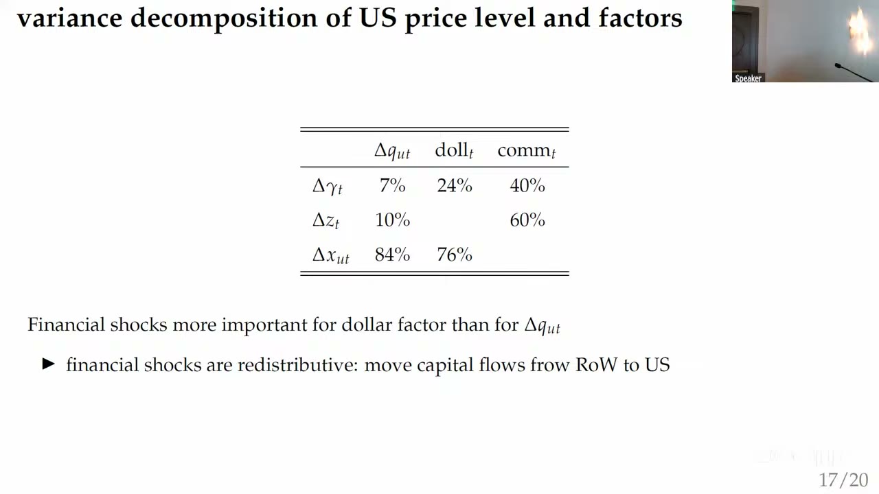
Here is the surprising number. In the calibrated model, $\gamma$ accounts for 7% of the variance of the us price, 24% of the dollar factor and 40% of the commodity factor. It redistributes without producing anything, and that is why: it pulls us and non-us prices in opposite directions, so it barely registers in a level and registers strongly in a relative price. Oskolkov’s gloss is that when the Australian dollar moves against the yen, part of that is commodity demand and part is intermediaries getting more frightened of commodity risk. These are model decompositions, not measured shock shares, and they are a statement about two relative prices rather than a claim that finance runs every currency.

They also rest on less than they seem to. A check of my own, not in the paper: under Proposition 4 the only source of factor covariance is $\gamma$, so the two $\gamma$ shares multiply to the squared factor correlation. Their product, $0.24\times0.40\approx0.10$, is therefore fixed by the data. The split between them comes from the externally set $\rho=2$. Re-solving Proposition 4 with the same moments and the same implied $e_H-e_L$, I get 15% and 66% at $\rho=1.25$, 31% and 32% at $\rho=3$, and 37% and 26% at $\rho=5$. The paper reports no such exercise. The us weight is another open dial: the model has the us equal to the rest of the world, Oskolkov put it nearer a third by gdp in their data, and said rescaling should preserve the results but that not every decomposition has been recomputed.

Three currencies

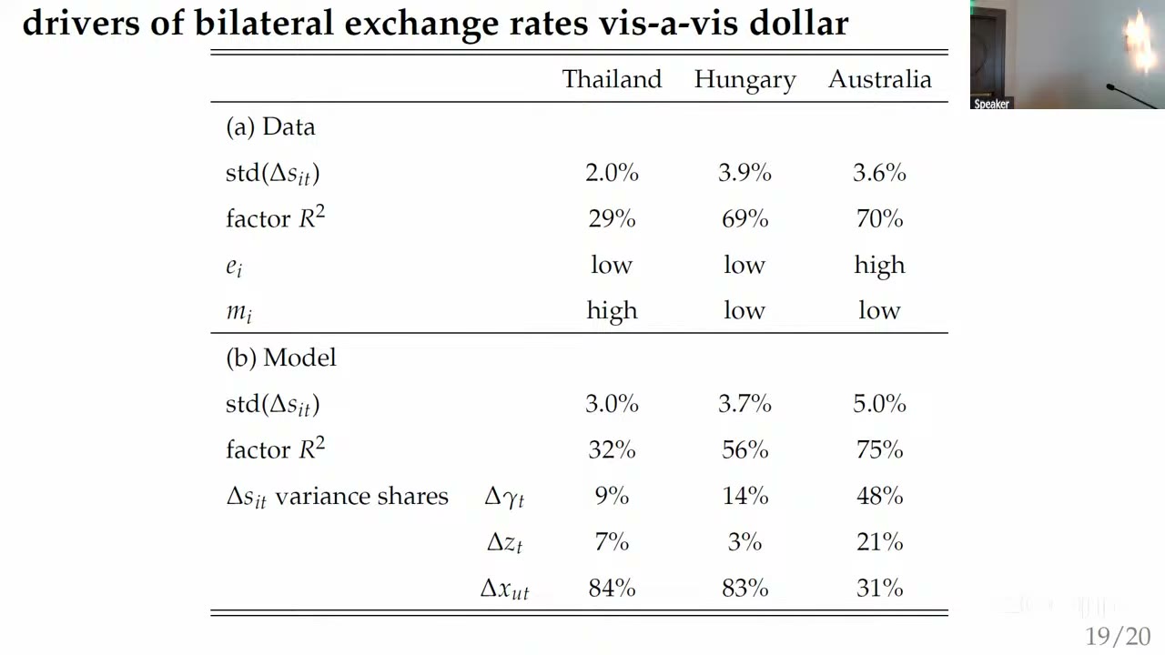
The payoff is a map of two coordinates. Thailand has low commodity exposure and high dollar assets; it is quiet, and most of what moves it is local. Hungary has low commodities and few dollar assets (Oskolkov suspects its foreign assets are mostly in euros), so us shocks go straight through. Australia has high commodities and low dollar assets, is exposed to both risks, and is where Oskolkov says financial shocks are nearly half of what global components explain.

Read that table carefully, because the shares do not say what they look like they say. Each column’s three numbers sum to 100 and exclude the local shock. So Australia’s 48% is a share of the global part. Multiply by the model $R^2$ of 75% (my arithmetic) and the risk shock is about 36% of Australian variance. For Thailand the local residual is about two-thirds. “Local” is itself assigned rather than measured, since everything the factors miss is ascribed to the non-tradable shock, and with one calibrated size for every country that shock alone is larger than Thailand’s entire exchange-rate volatility in the data. My guess is that this floor is why the model’s Thai volatility overshoots.

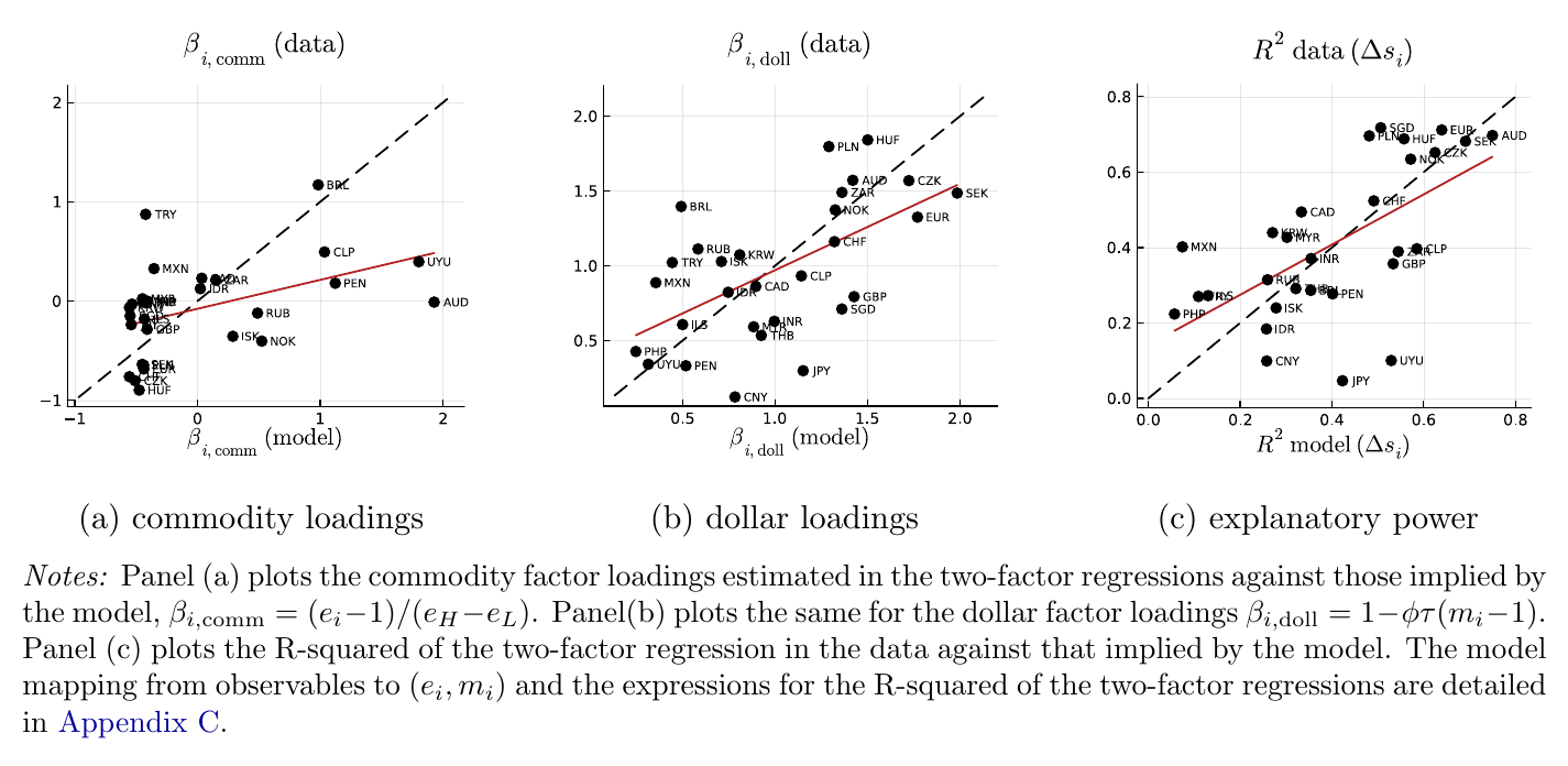
Now look at Australia in panel (a). It has about the highest commodity share in the paper’s scatter, it is the flagship commodity story, and its commodity loading in the data is about zero, against about 1.9 in the model, the worst miss in the panel. Its 70% data $R^2$ comes from a dollar loading of about 1.6. So the model gets Australia’s $R^2$ roughly right for a different reason than the data does, and overshoots its volatility on the way (5.0% against 3.6%). Norway, a commodity exporter on the model axis, has a negative loading in the data, and Turkey, which is not one, has a large positive loading. My tentative reading is that the commodity factor is sorting on something else as well, perhaps emerging against advanced, and the paper itself notes the overlap with carry. Thailand, meanwhile, is less hedged than advertised. Its model dollar loading is about 0.9, so on my reading its low factor $R^2$ owes more to low $e_i$ than to dollar assets, though Oskolkov credited the assets.

The discussant

Engel liked the framework and the empirical discipline, expects the paper to become a template, and said up front that the mechanism had not convinced them, while offering no alternative model. Engel also announced skipping the risk factor and the intermediary, so the paper’s most surprising number went undiscussed.

Five objections followed. First, are real exchange rates relative non-traded prices at all? In low-inflation, high-income countries Engel ties them to pricing-to-market and local-currency stickiness. The test: under a simple Balassa (1964)-Samuelson (1964) calibration the cpi real wage relative to the us should track the real exchange rate. In Engel’s quick detrended plots this is tolerable for Thailand and poor for Hungary and Australia, where the exchange rate swings about $\pm0.28$ and the wage about $\pm0.06$, read off the chart, and Engel called Australia typical of high-income countries.

Second, monetary stance. In Engel’s work with Wu, rolling 20-year $R^2$s reach about 0.28 with traditional variables around half of the fit, and Engel adds that a lot of these countries now target inflation. The paper has no monetary policy, so any such news lands in the residual.

Third, gross or net. The model runs on gross holdings because households can trade only local bonds, while Engel thinks net ought to matter for a wealth effect. A self-described rough calculation produced a correlation near zero, 0.036 or so. Treat this as provisional: Engel did not name the two variables (presumably the net ratio against the dollar loading), and Engel’s dollar shares differ from the paper’s. The paper’s nearest evidence does not settle it, because its nominally net series multiplies total net flows by a gross dollar share.

Fourth, intervention differed sharply across the three examples in 2008, and the model has a single $\tau$. (Australia intervened too and still fell most, so this does not simply rank them. Earlier, apparently on country-specific $\tau$, Oskolkov said there are too few data points to estimate one.)

Fifth, and sharpest: the whole channel is a wealth effect, and “the consumption literature doesn’t find big wealth effects.” Since $m_i$ is a share whose scale is fitted to the loadings, the paper has no independent check on that size. Engel still conceded that the correlation with dollar assets is there.

There is no reply. The recording of the Q&A is unusable, so no answer from the authors to Engel survives, and audience questions during the talk were off-mic, leaving only Oskolkov’s side of them. One of those answers deserves noting: on whether the sdf would stay so tied to global shocks if intermediaries consumed, which appears to be what was asked, Oskolkov said it needed more thought.

So the country the talk ends on is one with a commodity story and no commodity loading in the data, and, on Engel’s rough proxy, a non-traded-price story and no matching move in the wage. The fact underneath it, that dollar assets line up with dollar loadings, is still standing, and the discussant, whose job was to knock it down, said they had nothing to put in its place.

References