Some assorted notes on the ces-and-friends production functions that I came across.
1 Characterization of the standard ces
Definition
The standard ces utlity is of the form: \[ U(\mathbf{x}) = \left[ \sum_{i=0}^{n} \left( \beta_i \right)^{\frac{1}{\sigma}} \left( x_i \right)^{1 - \frac{1}{\sigma}} \right]^{\frac{\sigma}{\sigma-1}} \] where
- \( x_i \geq 0 \) is the consumption of goods \( i \in \mathcal{I} = \{1, 2,\dots, n\} \)
- \( \beta > 0 \) is the shift-share parameter of \( i \in \mathcal{I} \)
- \( \sigma \) is the constant elasticity of substitution
Let \( \mathbf{p} = (p_1, p_2, \dots, p_n) \) denotes the prices vectors. Budget constraint is \[ \mathbf{p} \mathbf{x} = \sum_{i \in \mathcal{I}} p_i x_i \leq E \]
Maximizing \( U(\mathbf{x}) \) over the budget constraint yield the ces demand: \[ x_i = \frac{\beta_{i} \left( p_i \right)^{-\sigma} E}{\sum_{k \in \mathcal{I}} \beta_{k} \left( p_k \right)^{1-\sigma}} = \beta_i \left( \frac{p_i}{P(\mathbf{p})} \right)^{-\sigma} U(\mathbf{x}) \] where \( P(\mathbf{p}) \) is the cost of living given by \[ P(\mathbf{p}) = \min_{\mathbf{x} \in \mathbb{R}^{n}_{ + }} \left\{ \mathbf{p} \mathbf{x} | U(\mathbf{x}) \geq 1 \right\} = \left[ \sum_{i=1}^{n} \beta_i (p_i)^{1-\sigma} \right]^{\frac{1}{1-\sigma}} \]
From these, the budget share for each \( i \in \mathcal{I} \) is \[ m_i \equiv \frac{p_i x_i}{E} = \beta_i \left( \frac{p_i}{P(\mathbf{p})} \right)^{1-\sigma} = \left( \beta_i \right)^{\frac{1}{\sigma}} \left( \frac{x_i}{U(\mathbf{x})} \right)^{1 - \frac{1}{\sigma}} \]
The indirect utility function are \[ U \left( \frac{\mathbf{p}}{E} \right) = \frac{1}{P \left( \frac{\mathbf{P}}{E} \right)} = \left[ \sum_{i=1}^{n} \beta_{i} \left( \frac{E}{p_i} \right)^{\sigma-1} \right]^{\frac{1}{\sigma-1}} \]
Properties
- Income elasticity of demand for each good is one , \( \frac{\partial x_i}{\partial E} \frac{E}{x_i} = 1 \), implying each good is neither necessary or luxury. This is due to its homotheticity.
- Marginal rate of substitution between any two goods, and hence their relative inverse demand, \( \frac{p_i}{p_j} = \frac{\partial U(\mathbf{x})}{\partial x_i} \big/ \frac{\partial U(\mathbf{x})}{\partial x_j} = \left[ \frac{x_i / x_j }{\beta_i / \beta_j} \right]^{- \frac{1}{\sigma}} \), is independent of the quantity of a third good. This is due to the directly explicit additivity (dea) of ces. Furthermore, \( x_i \) and \( x_j \) enter only as their ratio \( \frac{x_i}{x_j} \).
- Relative demand between any two goods, \( \frac{x_i}{x_j} = \frac{\beta_i}{\beta_j} \left( \frac{p_i}{p_j} \right)^{- \frac{1}{\sigma}} \), is independent on the price of the third good. This is due to the indirectly explcit additivity (iea) of ces. Furthermore, \( p_i \) and \( p_j \) enter only as a ratio, \( \frac{p_i}{p_j} \).
- The elasticities of substitution between all pairs of goods are identical across all pairs, and the price elasticity of demand for each good, holding \( P(\mathbf{p}) \) fixed, is constant and identical.
- All goods are either
- gross complements (i.e. \( m_i \) is increasing in its relative price \( p_i / P(\mathbf{p}) \), for \( \sigma < 1 \)
- gross substitutes (i.e. \( m_i \) is decreasing in its relative price \( p_i / P(\mathbf{p}) \), for \( \sigma > 1 \)
- If the goods are gross substitutes, they cannot be essential ender ces.
- No choke price: Demand for any good remains strictly positive when its relative price becomes arbitrarily high
- Non-satiation: Demand for any good goes up unbounded when its relative price becomes arbitrarily low
- with \( \sigma \neq 1 \), one could set \( \beta_i = 1 \) by choosing the unit of measurement of each good appropriately; the standard ces can be assumed to be symmetric without loss of generality.
2 Variants
Nested ces
In any multi-sector models, where the intersectoral demand is given by the representative consumer with ces preferences, and each sector produces its output using a ces production function or a variety of goods aggregated by ces, such as multi-sector Eaton and Kortum (2002), models by Costinot et al. (2012) and Caliendo & Parro (2015), effectively use nested ces.
Deviate from dea and iea
Deviate from dia, iia and implicit ces
- Implicit additivity is the weaker version of explicit additivity.
- Non-homothetic ces satisfies both dia and iia
- Is commonly seen in the literature of structural transformation
Homothetic non-ces
- crs \( \rightarrow \) linear homogeneity \( \rightarrow \) homothetic.
- A function is said to be linearly homogeneous (or homogenous of degree one) if doubling, tripling, or otherwise uniformly scaling all of the inputs results in the output being scaled by the same factor. Mathematically, if \( F \) is a production function and \( k \) is a positive scalar, a function \( F \) is homogeneous of degree 1 if \( F(kx, ky) = kF(x, y) \) for all \( x \) and \( y \). This property is significant in economics because it indicates constant returns to scale.
- A function is said to be homothetic if it is a monotone transformation of a homogeneous function. In other words, a function is homothetic if it can be composed of a homogeneous function and a monotonic function. In economic terms, homothetic preferences or production functions are useful because they imply that the mix of goods chosen by a consumer, or the mix of inputs used by a producer, does not depend on the scale of operation but only on the relative prices of the goods or inputs.
Homothetic Indirect Implicit Additivity (hiia)
3 Visualizations
Homotheticity
A homothetic function exhibit the same shape of contour lines.
import numpy as np
import matplotlib.pyplot as plt

# Define the range of values for K and L
max_values = [10, 50, 100]

# Populate grid values
Fs = []; Ks = []; Ls = []
for max_value in max_values:
    K, L = np.meshgrid(np.linspace(0.1, max_value, 100),
                       np.linspace(0.1, max_value, 100))
    F = K**0.7 * L**0.4
    Ks.append(K); Ls.append(L); Fs.append(F)

# Create the subplots
fig, axs = plt.subplots(1, 3, figsize=(20, 5))

for i, ax in enumerate(axs):
    c = ax.contourf(Ks[i], Ls[i], Fs[i],
                    vmin=Fs[-1].min(), vmax=Fs[-1].max(),
                    cmap='coolwarm')
    fig.colorbar(c, ax=ax)
    ax.set_title(f'Zoom view: [0- {max_values[i]}]')

plt.show()
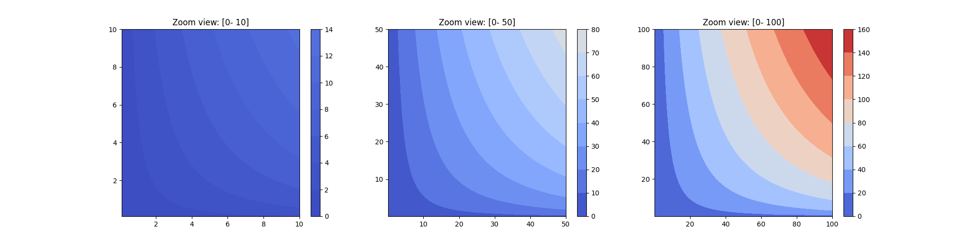
Figure 1: Contour plots for ( F(K, L) = K^{0.7}L^{0.4} ), at different zoom levels, showing the same contour shapes