Networks, Barriers, and Trade

David Baqaee (UCLA) and Emmanuel Farhi (Harvard; died July 2020). The version of record is the Econometrica article, 92(2), 2024, pp. 505–541, and that is the document this digest reads. The proofs are not in it: they sit in an Econometrica Supplemental Appendix, which is not in hand. The extended appendices E–M — the non-nested-CES generalization, the trade elasticities, the factor demand system, the all-country growth accounting — exist only in the superseded NBER working paper 26108, which the published text repeatedly points to but which is likewise not read here. No talk recording could be found; PDF-only digest. Figures 2 and 4 are cropped from the published article.

A map of territory usually explored by machines

Quantitative trade models with input-output linkages are solved on computers, and the complaint the paper opens with is that when the computer returns a number nobody can say which force produced it. The paper’s ambition is to write down, for a very general class of such models — many countries, many sectors, arbitrary nested-CES production and consumption, any pattern of trade, and any “wedges” (tariffs, markups, sticky prices) — the first-order response of every price, quantity, real GDP and welfare to any shock, and the second-order response of world welfare and of real GDP around efficiency, as explicit functions of the input-output matrix, the elasticities of substitution, and the wedges in the initial equilibrium. The second-order half is deliberately narrower than the first: footnote 25 on p. 524 says the paper does not provide second-order approximations for country-level welfare, except in symmetric cases where country and world welfare coincide, nor for real GDP away from efficiency, because both would require superelasticities — elasticities of elasticities of substitution. Within those limits it is hat-algebra for the world with networks in it. The payoff for geoeconomics is that “what does it cost to cut country X off from input Y” becomes a question with a formula behind it, and the formula tells you which features of the economy make the answer large.

Two decompositions and a propagation theorem

Theorems 1 and 2 are ex-post accounting. The change in a country’s real GDP splits into a technology term — the shock weighted by Domar weights, holding the allocation fixed — and an allocation term that vanishes in the absence of domestic wedges in the initial equilibrium (Corollary 1), and otherwise tracks reallocation toward high-marginal-value uses through changes in factor income shares. The condition is domestic wedges, not efficiency at large, which is what makes Theorem 1 a country-level result: a country with clean domestic markets sitting inside a thoroughly distorted world still gets the corollary. For welfare the reallocation term survives even in efficient economies, and it depends on what the paper calls the factoral terms of trade: how the shock moves the prices of the factors a country sells to the world relative to those it buys. This is the open-economy sense in which a foreign productivity shock leaves a country’s real GDP unchanged (Theorem 1) while changing its welfare (Theorem 2).

Theorem 3 is the engine. For a vector of productivity and wedge shocks, it gives the first-order change in every price and sales share as the solution of a linear system built from the input-output matrix, elasticities and wedges. Iterating it — integrating the differential system rather than solving the nonlinear excess-demand system once — gives exact nonlinear counterfactuals, and is faster for large highly nonlinear models. Extensions handle endogenous factor supply, sticky wages with an inflation-targeting central bank, and sticky prices.

Losses from barriers are Harberger triangles, Domar-weighted

Section 5 gives the second-order results. Starting from an efficient equilibrium, the real GDP loss from introducing small tariffs or other wedges is

(Theorem 5): a sales-weighted sum of deadweight-loss triangles, each the product of the wedge and the quantity response it induces, with the quantity responses themselves given by Theorem 3 in terms of primitives. Two things follow. Because Domar weights include intermediate sales, they sum to more than one, so barriers on inputs matter more than their value-added share suggests. And the loss is second-order in the wedge, so small barriers are nearly free while large ones are not — the same convexity as in the authors’ Beyond Hulten’s Theorem, now for trade.

The analytical examples

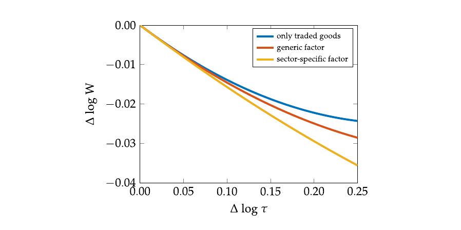
Section 6 works four stylized cases that carry the paper’s message. With input-output linkages, goods cross the border more than once, and the first-order welfare elasticity to an iceberg shock is trade as a share of GDP — not trade as a share of sales, which is the ratio a calibration without linkages preserves, and which is smaller by roughly the ratio of sales to GDP, about two. With domestic complementarities across sectors (elasticities below one), a large negative trade shock is much costlier than a Cobb-Douglas calculation implies, because the domestic economy cannot reallocate to replace the lost imports — the paper names the German gas debate (Bachmann et al. 2022) as the case in point. With factors specific to sectors, the complementarity bites harder still, and Figure 2 is the demonstration. The import share of consumption is pinned at one sixth in all three specifications, so the three curves are first-order identical by construction and the ACR sufficient statistic cannot tell them apart; what the chart shows is the three economies separating purely in the second-order term, over a range that stops at a change in log $\tau$ of 0.25 and never comes near autarky. The one-sector curve flattens and ends near a 2.4 percent welfare loss; the generic-factor curve is close to linear at 2.9 percent; the sector-specific curve is the steepest and still steepening at 3.6 percent, half again as costly as the case the ACR formula prices. Example III turns on sticky wages: symmetric countries, floating rates, wages rigid in domestic currency with capital flexible, and every central bank targeting zero domestic inflation. The trade shock raises consumer prices, the bank contracts nominal spending to hold the price level, the contraction falls on employment one-for-one because nominal wages cannot move, and equation (16) prices the result — the direct effect of the shock divided by one minus labor’s share of income, so the losses grow with the sticky factor’s share. Example IV is a different economy, and it is the one aimed at Fajgelbaum et al. (2020): two asymmetric countries, one factor each, wages downwardly rigid in both, the foreign country pegging its exchange rate to the home currency while the home country targets zero inflation. Under flexible wages a well-designed tariff turns the factoral terms of trade in America’s favor and pass-through is therefore incomplete; under the rigidity and the peg, equation (19) drops the factoral terms-of-trade term out of the welfare change entirely, which is why pass-through is complete, and why the American welfare gain is zero to first order when the taxed goods are consumed domestically rather than reexported.

The quantitative check

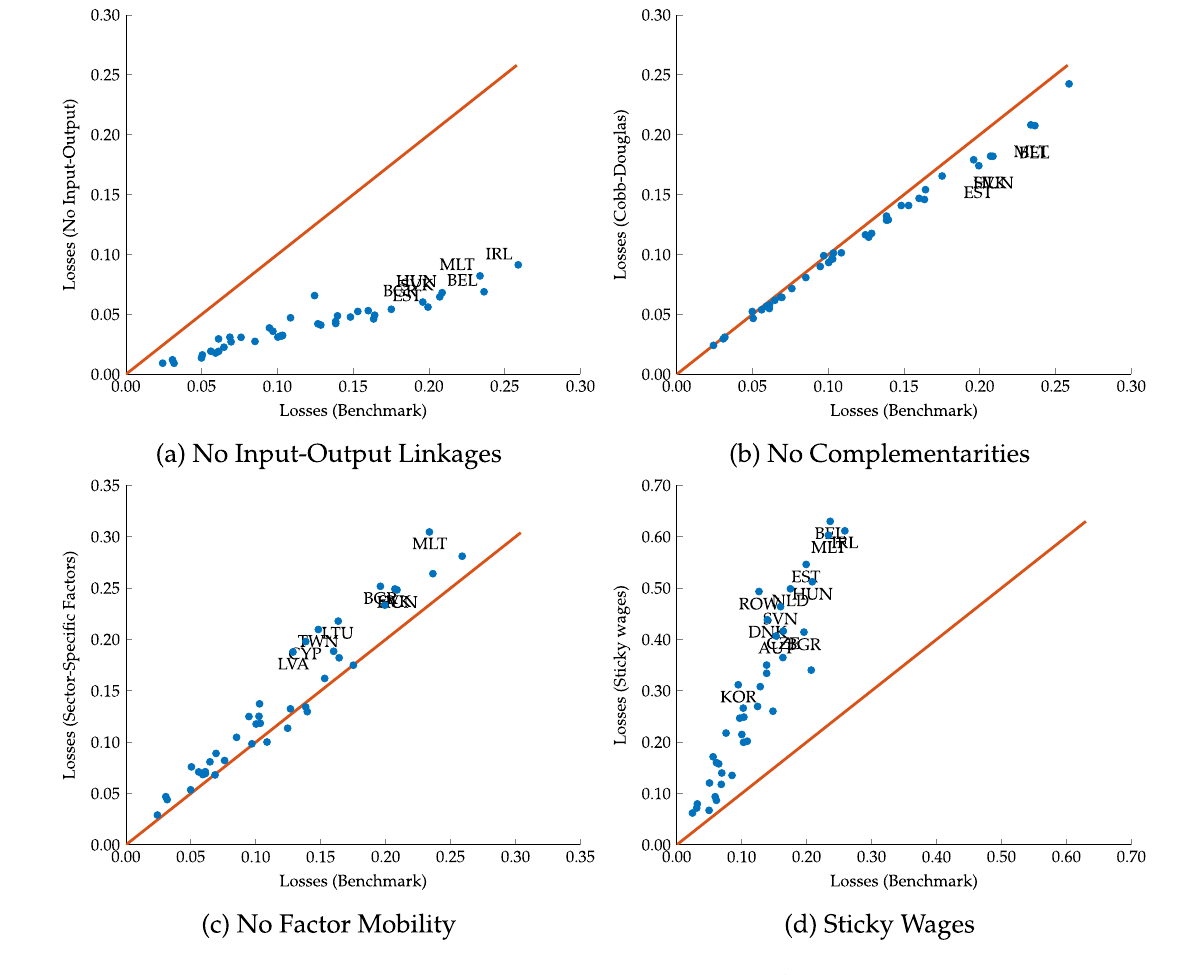
Section 7 calibrates a multi-country, multi-sector model to world input-output data and runs a 60 percent universal increase in trade costs — a fragmentation shock of the kind the IMF scenario papers use. The four panels of Figure 4 are the analytical examples in data. Linkages are a first-order effect that doubles losses for everyone; complementarities and factor immobility are second-order effects that matter for open, imbalanced economies (Malta, the Baltics, Taiwan, Eastern Europe) and would matter more for shocks closer to autarky; nominal rigidities are first-order and double losses again. The growth-accounting half of the section decomposes real GNE growth into technology and reallocation terms for two countries, the United States and Italy.

Two decompositions, one country, opposite signs

Those two countries are chosen to make a point that is easy to miss and hard to unsee. The conventional Dixit-Norman decomposition, equation (6), splits welfare into real GDP plus the goods terms of trade; Theorem 2 splits it into technology plus the factoral terms of trade. Run on American data the two agree. Run on Italian data over the same years they disagree about the sign of what happened. The conventional split says Italian real GDP grew far more slowly than Italian real GNE and attributes the gap mostly to an improvement in the terms of trade, the price of the foreign goods Italians consume having fallen relative to the price of what Italy exports, which reads as good news. Theorem 2 says Italian consumption grew more slowly than the technology embodied in the goods Italians consume, and attributes that gap to a deterioration in the factoral terms of trade. The paper’s own gloss, on p. 536: “Intuitively, the right panel tells us that foreign factor rewards outpaced Italy’s factor rewards, and this implies that Italy is consuming a smaller share of a bigger global pie.” Same data, opposite story, and the paper says plainly on p. 518 that the factoral terms of trade need not share the sign or the magnitude of the standard ones.

The argument for preferring the factoral measure is made on that same page and it is the one a geoeconomics reader should keep, because it is about what the statistic responds to. Whether an iceberg trade cost is logged in the importing country or the exporting one has no bearing on any equilibrium allocation or on anyone’s welfare, but it does change measured real GDP, and therefore the measured terms of trade, since the two must sum to the change in welfare. The same goes for a firm that changes the country where it books its profits: the goods terms of trade move, and Theorem 2’s factoral terms of trade do not. A measure that responds to where a multinational puts its tax domicile is a poor foundation on which to run trade policy.

Where it sits

This is the workhorse behind every decoupling counterfactual and the reason the production-network papers belong in a geoeconomics list. The CMS hegemon’s power runs through the Leontief inverse; Liu–Yang’s measure weights import shares by elasticities; the IMF’s fragmentation cost scenarios are Theorem 3 iterated. What this paper supplies is the statement of which primitives the answer depends on — the IO matrix, the elasticities at each nest, the wedges, the factor-mobility assumption, the nominal regime — and the warning, made concrete in Figure 4, that a model missing linkages or nominal rigidities will understate the cost of a trade disruption by a factor of two, while a model with Cobb-Douglas domestic sectors will understate the cost of a large one. Read it after Beyond Hulten and before Bachmann et al., which is the case where these choices were made in public under a deadline.