The Very Long-Run Costs of Financial Crises

Karsten Müller, Chenzi Xu and Mohamed Lehbib, presented by Xu at the nber International Finance and Macroeconomics Program Meeting, 23 October 2026; discussant Sanjay Singh. No public paper exists, so this note rests on the talk and its slides alone and is flagged as such; values read off a chart are marked approximate.

You want to know what a banking crisis costs. So you compare a country’s output after the crisis with what it would otherwise have been, and you keep comparing until the data run out, which in most of the literature is around year five. Now you have a problem, because the size of the bill depends on what happens after you stopped reading it. If output plucks back to trend, the crisis was a bad few years. If it never does, the crisis was a permanent tax. The first five years of those two worlds can look alike, and the deck’s motivation for caring is the obvious one: “larger output losses justify more ex ante intervention.”

Anyway, Müller, Xu and Lehbib went and got the rest of the bill. The reason nobody had much of it is that a fifty-year impulse response needs very long series for many countries, and banking crises are rare. So they built the Global Macro Database: 239 countries and territories, 167 sources, 46 variables, ratio-spliced onto one another, with 368 crisis onsets taken as the union of four existing chronologies. It is an enormous public good, and it is in service of what Xu cheerfully called “a paper that primarily has one result.” (Those are database-wide counts. No regression sample size is printed anywhere in the deck, so how many crises identify year 39 is not something this note can tell you. Crises are also 0/1, and when someone in the room objected that this treats svb and Lehman alike, Xu agreed.)

The regression

There is no model, and the authors say so: “Rather than estimating a structural model, we provide reduced-form evidence on plausible channels.” The whole apparatus is a panel local projection, from the deck’s slide 21:

Here the left side is the long difference in log real gdp from $t-1$ to $t+h$, the $\Delta$ in the lag terms is one-year growth, BankingCrisis is 1 in a crisis’s first year, $\beta_h$ is the output gap $h$ years on, $\alpha_i^{(h)}$ is a country fixed effect, and $L = 25$. It is run separately for $h = 0,\dots,50$, so nothing imposes persistence. The counterfactual is not a drawn trend line (the opening pictures of the us and uk falling below trend are motivation only) but the country’s own conditional growth over that horizon.

The one result

At year ten the authors have gdp 7.0 percent lower in the full panel and 9.1 percent lower in the balanced panel. Other studies, precision-weighted, say 6.7. So far nobody is disagreeing with anybody. Then the point estimates keep falling: to 12.1 percent at year 39 in the full panel, and to 17.2 percent at year 31 in the balanced one.

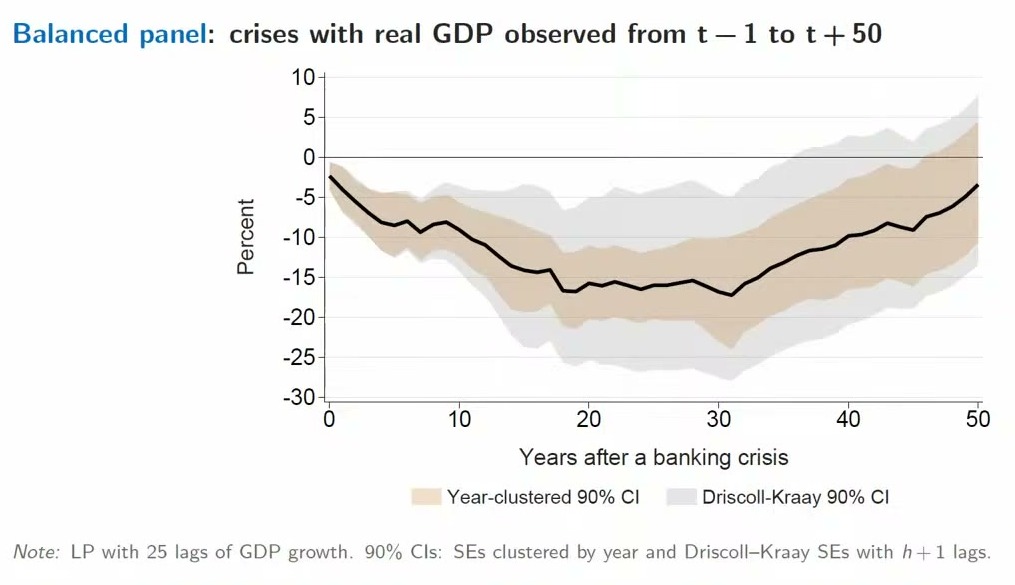
That is the surprising thing, and it is a slightly funny kind of surprise, because the authors do not contradict anyone about any year anyone measured. Of the fifteen studies on the comparison slide, the median peak comes at year 4 and the latest at year 8. Xu’s account of the gap is that “most of these papers don’t go out far enough.” The hole does not merely fail to fill; on these estimates, which are averages over crises, it keeps getting deeper for twenty-odd years after the literature went home. And Xu concedes the awkward part: whether a crisis lasts one year or five, “it’s hard to sort of explain” thirty.

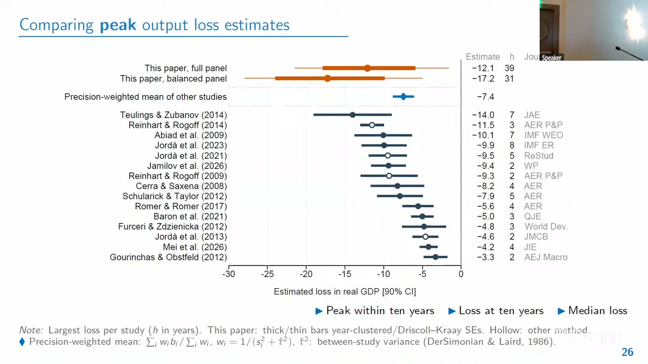
Keep the two numbers apart. The headline “17 percent” is the balanced panel, which needs each crisis observed for the full fifty years, so recent crises drop out by construction (Singh gives the last onset as 1975). Xu reads the gap between panels as “more recent crises, especially in the shorter term” being less severe. Xu’s claim of larger losses than all other estimates holds for 17.2; the full-panel 12.1 is smaller than Teulings and Zubanov (2014)’s 14.0. And the slide’s “remain lower for five decades” is a statement about point estimates: by year 50 both panels sit near -3.5 (a chart read) and neither panel’s 90 percent bands exclude zero.

The table

The authors prefer Driscoll-Kraay (1998) errors, whose intervals run up to twice as wide as year clustering, and call them conservative. Now look at their robustness table with that column in mind.

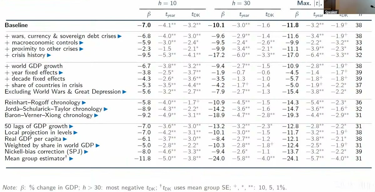
The baseline at year 30 is -10.1 with $t_{DK} = -1.6$: no star. The far-horizon baseline, which picks the horizon by its $t_{DK}$ rather than its depth, gets to -1.9, a 10 percent star. Xu described the drift after year ten as “not in a super significant way.” Some rows push the other way, hard: crisis history -17.2, Baron-Verner-Xiong (2020) dates -18.9, the mean-group estimator -24.0. But add year fixed effects and year 30 goes from -10.1 to -1.9, with $t$-statistics of -0.7 and -0.6. Decade effects give -3.5; the share of countries in crisis gives -4.2. Year 10 under year effects is about halved and still significant, so what the control eats is largely the part that was news. The closing slide says losses stay lower for decades “across controls, samples, and estimators,” and these three rows are the exception.

A questioner raised this, and Xu had an answer. The worst crises are global ones (2008, 1931, 1907), a year effect absorbs exactly that, so “this is basically overcontrolling,” and the attenuation is “kind of nice evidence.” This is a coherent argument and it is not a test. It works only if the global component is part of the crisis rather than a common shock that happened to coincide with it. And controlling for world gdp growth, which is the same worry in another form, leaves -9.4, a gap the talk did not resolve. A randomized-crisis placebo was mentioned and not shown.

The rest of the floor’s mid-talk questions, from people the recording cannot name, went at the object itself. Is the pre-crisis path the right benchmark, if some of those economies were overaccumulating? The authors take no stand: “we don’t do anything with welfare.” Is a fast grower’s slowdown after a crisis the crisis or just development? “We haven’t done anything like that.” Would V-shaped crises of varying length average into something that looks permanent? Not done. Why would one coefficient hold across two centuries of changing policy and banking? Emerging-versus-advanced splits show little heterogeneity, Xu said, though the historical measures of financial depth were poor. Underneath all of it, crisis onset is not randomized, and the rows of the table address observable confounders, not whether every later loss was the banks’ doing.

What might be doing it

The channels are more impulse responses, not a decomposition, and “consistent with” is the honest verb. Investment falls about 15 percent within three years, three times consumption, and stays about 10 percent below path for three decades, before rebounding late. Capital per worker, a technology-adoption score, output per hour and years of secondary schooling all sit lower for decades, on chart reads, and revenue over gdp falls while debt over gdp rises and later reverses. Less investment means less output is a story the room can tell itself. Two limits: the capital and productivity panels start in 1950 and stop at year 30, so they cannot speak directly to the older crises in the balanced cohort, and nothing splits the loss across channels.

The discussant

Singh’s first question was why anyone should care about year 39, and the answer is a welfare calculation, his own and not the authors’. Take log utility, a 3 percent annual crisis probability and a discount factor of .96, and from his slide 4 the permanent consumption you would give up to avoid crises is

where $p$ is the crisis probability, $\theta_h$ the log impulse response at horizon $h$ with gdp standing in for consumption, and $\beta$, confusingly for present purposes, the discount factor rather than the regression coefficient. Lucas (2003) got 0.05 percent for business cycles. Singh takes the Jordà-Schularick-Taylor response through year ten and attaches three tails.

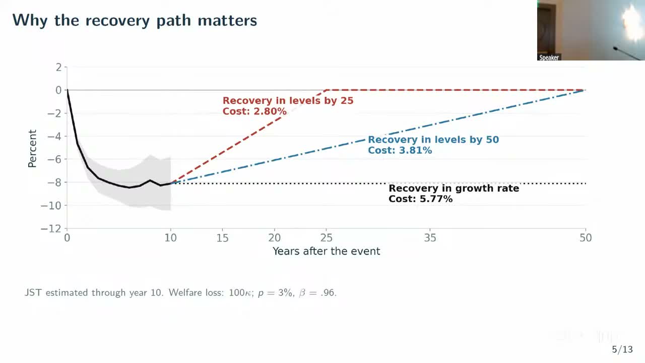
So the tail is worth a factor of two, which is the paper’s case. Then he takes it back a little. Run the authors’ balanced response through the formula and you get about 5 percent, close to what you would get by stopping at year ten and assuming no level recovery. Discounting is why: $.96^{25}$ is .36 and $.96^{50}$ is .13, so knowing the path “up to year 25 is more or less enough.” The fifty-year panel’s main welfare contribution is telling you what years 10 to 25 look like, which the long-standing advanced-economy dataset, down to 24 crises by then, cannot. The sample moves things more than the far tail does: on his calculations the same data give 5.28 percent with 152 crises at every horizon, and 3.64 percent if later crises fill in the intermediate horizons (293 at year 25), the extra 140 or so being heavy with quick-recovering emerging markets. That sits awkwardly with Xu’s report of little emerging-market heterogeneity, and neither side put numbers on it.

His second question was whether the confidence bands mean anything out there. In a random walk with an observed shock, the true response is 1, but $\hat\beta_h - 1$ is of order $\sqrt{h/(T-h)}$ because later shocks line up with the first one by chance, so stretching the horizon along with the sample can eat the gain.

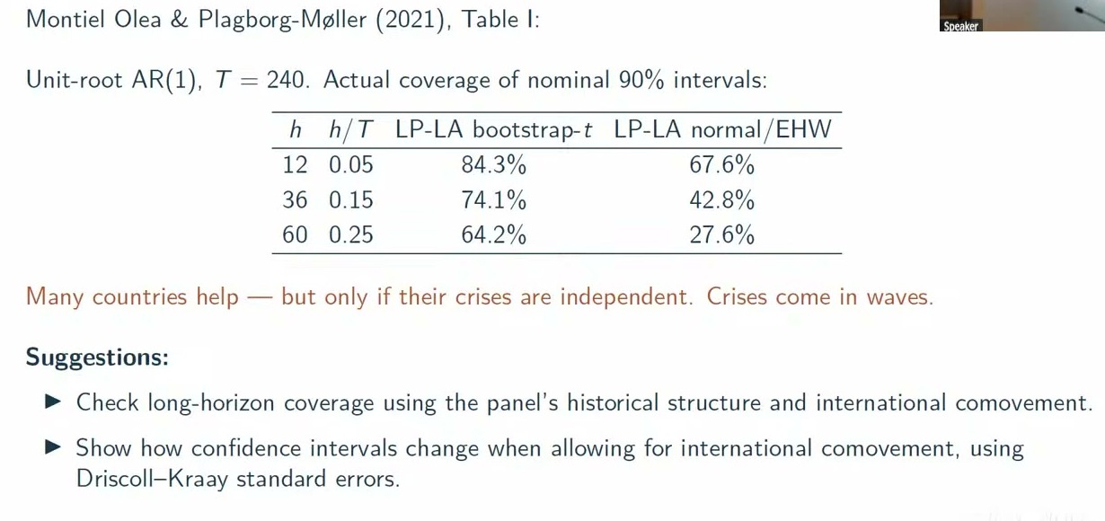
At $h/T$ of 0.25, a nominal 90 percent interval covers 64.2 percent of the time with a bootstrap and 27.6 percent with normal errors. His mapping puts year 50 over 150 years of data at 0.33, off the end of the table. This is one univariate data-generating process, not a finding about this panel. But many countries help only if their crises are independent, and, as the slide puts it, “crises come in waves.” He counted about 18 countries back to 1800 and 34 to 45 from 1920, so roughly an 80-year window in which you “basically have one or two observations.” (Wider is also not the same as correct: Driscoll-Kraay answers the correlation, not the coverage.) He asked for two things. Show Driscoll-Kraay intervals, which the authors have added since the draft he read; and simulate long-horizon coverage from something that keeps the panel’s structure, which is not in the talk.

The recording has no author reply to any of this: the chair thanks Singh, then laptop trouble and the changeover take over, and no floor discussion survives. Singh’s last slide also refused to appear, so his closing aside, that banking crises have very persistent effects on judicial freedom while wars do not, comes from speech alone and has no figure behind it.

The closing slide’s policy line is careful, and it should be: crises “might not be a price worth paying for faster growth.” The authors built a database that starts in 1086 to find out what happens around year 39, and a discount factor of .96 gives year 39 a weight of about a fifth. But the argument that survived the session is over whether crises cost 3 percent of consumption forever or 5, and if you were raised on 0.05, that is a remarkable thing to be arguing about.

References