Uneven Growth: Automation's Impact on Income and Wealth Inequality

Benjamin Moll (lse), Lukasz Rachel (ucl) and Pascual Restrepo (bu). Presented by Moll at caffe, the cepr Advanced Forum in Financial Economics, on 8 February 2022; discussed by Laurent Calvet (edhec), with questions afterwards. This is the published Econometrica version, November 2022 (vol. 90, no. 6, 2645–2683).

The automation in this paper is almost incidental. What is load-bearing is a slope.

Start where the literature starts. In the neoclassical growth model the long-run supply of capital is a horizontal line at the discount rate: households will hold any quantity of capital you like, forever, at $r = \rho$, and not a basis point less. Shift capital demand right however you please — automate every routine task, invent the robot, hand capital a larger Cobb–Douglas exponent — and in the long run the price of capital does not move. All you get is more capital. And if the rental rate doesn’t move, then by the dual Solow residual the entire productivity gain has to land somewhere else, and there is only one somewhere else: wages. That result is old and robust, and it is why a large and careful literature on automation is a literature about relative wages. Technology can reshuffle who gets what inside the labour share; it cannot stop the labour share from collecting.

Moll, Rachel and Restrepo tilt the line. Everything else in the paper follows, and the following is elegant enough that Moll says so out loud at the whiteboard moment of the talk: “Once you understand this, this is really you almost understand everything that’s there in the paper, because everything else follows logically from this.”

The wedge, and what it costs

To tilt the supply curve you have to break Gorman aggregation, because a model that aggregates has an indeterminate wealth distribution and a return pinned at $\rho$. The paper breaks it with dissipation shocks: at Poisson rate $p$, a household’s financial wealth goes to zero and it starts again on its labour income. The effective discount rate becomes $\rho = \varrho + p$; set $p = 0$ and every formula in the paper collapses back to the representative-household benchmark, which is exactly why Moll uses it as the organising device of the talk.

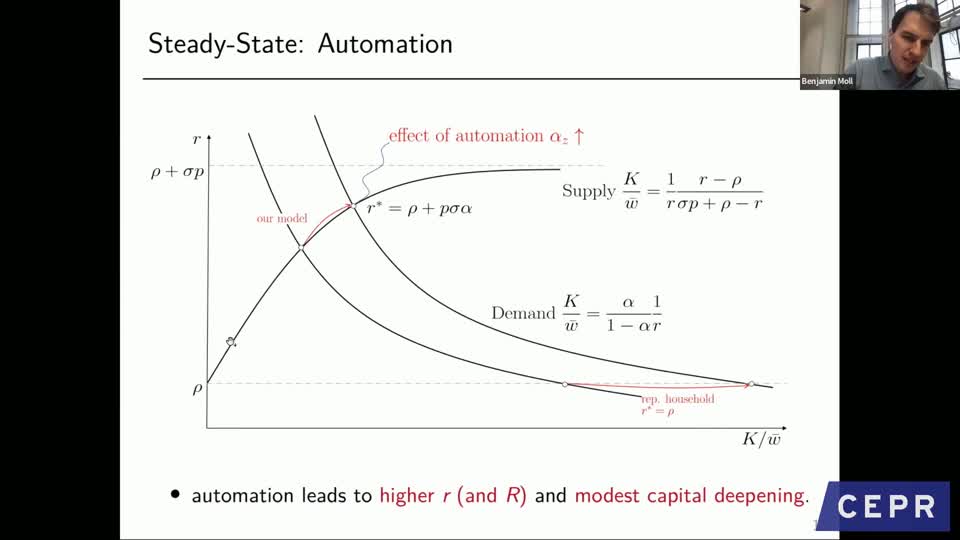
Now everything happens on one diagram. Normalise capital by the wage bill, $k = K/\bar{w}$. Capital demand slopes down. Capital supply now slopes up and, more usefully, is bounded: it leaves the axis at $r = \rho$ and asymptotes at $\rho + p\sigma$, so the equilibrium return is trapped in that interval. Automation raises the share of tasks machines can do, which raises the Cobb–Douglas exponent on capital, which shifts demand right. Against a flat supply curve that is a quantity event. Against this one it is partly a price event, and the price has a closed form — equation (5), p. 2653:

Here $r^*$ is the steady-state return to wealth, $\rho$ the effective discount rate, $p$ the dissipation rate, $\sigma$ the inverse intertemporal elasticity of substitution, $\alpha^*_{\mathrm{net}}$ the net capital share, $K^*$ the capital stock and $w^*_z$, $\ell_z$ the wage and population share of skill $z$; at $p=0$ the last term vanishes and you are back in Ramsey.

One piece of notation deserves to be caught in the act, because the whole paper is routinely misread through it. That $\sigma$ is the inverse ies, calibrated at 2. It is not a capital–labour elasticity of substitution. Production here is Cobb–Douglas at the sector level, so the elasticity of substitution between capital and labour is exactly 1, by construction, and nothing in the argument rides on it. The capital share rises because tasks are reallocated from workers to machines, not because a ces parameter exceeds one. Whatever you think of the contested $\sigma_{KL} > 1$ literature, this paper is not in it.

Note also what equation (5) does not depend on. It drops straight out of the steady-state condition $0 = \dot{K}$ for any constant-returns technology, so any change that raises the net capital share raises the return to wealth. Automation is the paper’s subject, but it is not privileged by the mathematics.

From a factor share to a personal distribution

Define effective wealth $x_{zt} = a_{zt} + w^*_z / r^*$, financial plus human. Between shocks it grows at the constant rate $(r^*-\rho)/\sigma$; at rate $p$ it resets to the human-wealth floor. That is random growth with reset, the Champernowne/Wold–Whittle machine, and its stationary distribution is exactly Pareto with tail index equal to the ratio of the accumulation rate to the reset rate — which in equilibrium is $\alpha^*_{\mathrm{net}}$.

So in the baseline model the tail index of the personal distribution of wealth and income equals the factor share of capital. Raise automation, raise the capital share, fatten the tail, and top income inequality rises with no change whatsoever in the wage distribution required. That is a genuinely pretty result and it deserves its caveat immediately: it is the baseline one-asset, zero-growth statement and nothing wider. Once the economy grows the net share is redefined net of growth as well as depreciation and taxes, and once capital returns are risky the tail formula is replaced outright and the tail index strictly exceeds $\alpha^*_{\mathrm{net}}$. This matters a lot quantitatively, and the paper says so: the baseline delivers a tail index of about 0.2 against empirical values around 0.7. The analytically beautiful version of the result cannot match the data it is about. The extended model with idiosyncratic capital risk gets to 0.66, and that is the model that gets calibrated.

This is also, emphatically, not the Meade–Piketty compositional argument that a bigger capital share raises inequality because capital income is more concentrated than labour income. The paper decomposes and prices that channel: for the us top 1% in 1980, a one-point rise in the net capital share raises the top-1% share by 0.07 points, against an observed rise from 10% to 20%. The compositional effect is real and it is a rounding error. The new channel is the within-factor term — automation makes capital ownership more concentrated, because everyone who owns capital now compounds faster.

The flip side, which is the title

The other arm is the dual Solow residual, equation (10), p. 2656:

$d\ln\mathrm{TFP}_\alpha$ is the productivity gain from automating more tasks, $\alpha$ the gross capital share, $\bar{w}$ the average wage, $R$ the rental rate and $\delta$ depreciation. There are two doors and no third one. With perfectly elastic capital supply, $d\ln R = 0$ and every gain walks out through wages. Tilt the supply curve and some of it walks out through $R$ instead.

How much is “some”? Enough to matter, because of an arithmetic asymmetry that footnote 20 lays out with no ceremony. At a 1980 capital share of 0.345 and a rental rate of 11.5%, a one-point rise in $R$ is a 10% rise in $R$, so $\alpha \, d\ln R \approx 3.45\%$ — larger than the 2.5% tfp gain the calibrated shock produces. The residual for wages is about minus one percent. Small movements in returns eat large movements in productivity, because returns are a small number and shares are not.

Hence Proposition 2, and it is a threshold result, so state it as one. Automating skill $z$’s tasks always lowers $w_z$ relative to other wages. But for the average wage there exists a $\bar{p} > 0$ such that automation lowers $\bar{w}$ when $p > \bar{p}$ and raises it when $p < \bar{p}$ — a race between the displacement term and the output expansion, as Calvet restated it cleanly in the discussion: automation “can decrease the average wage if $p$ is sufficiently high… if capital gets destroyed sufficiently fast.” Automation raising tfp and output while permanently lowering the real wage is something this model can do, conditionally. It is not something automation does.

The calibration, and what it is a calibration of

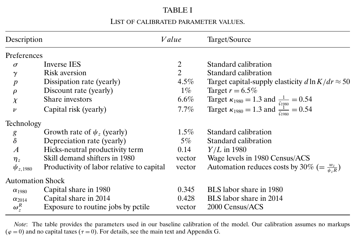
Table I sets $p = 4.5\%$ a year, $\rho = 1\%$, a 6.6% share of households permitted to hold equity, idiosyncratic capital risk $\nu = 7.7\%$, and an automation shock that moves the bls capital share from 0.345 in 1980 to 0.428 in 2014, apportioned across 100 wage percentiles by exposure to routine jobs. Markups and capital taxes are switched off. Which means the exercise attributes the whole labour-share decline to automation by assumption, and the paper says so in as many words: the calibration asks what would follow if the observed decline in the labour share were explained by the automation of routine jobs. It is a conditional experiment, not a measurement.

Two things about that dissipation rate are worth noticing. It is calibrated to a capital-supply semi-elasticity $d\ln K / dr$ of about 50, and the paper calls this conservative — because the published estimates it surveys all sit below 35, and a less elastic capital supply would make every distributional result in the paper larger. That is an unusual direction for a robustness argument to run. And the whole apparatus is, as Moll cheerfully concedes, a stand-in: “it’s a stand-in, right? For other things that give you a non-degenerate wealth distribution and upward-sloping capital supply.” Aiyagari-class models have both features honestly, “but you can only solve them on a computer… we wanted to have something essentially that functions basically like an Aiyagari model but which you can solve with pencil and paper.”

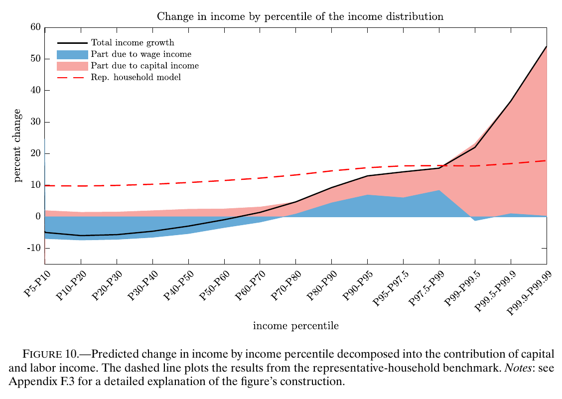
What comes out is Figure 10, comparing steady states: incomes fall 5–10% below the median, stagnate from the 50th to the 80th percentile, rise 20% for the top 1%–0.5% and 55% for the top 0.1%. Feed the identical shock to a representative-household version and you get a fairly uniform gain of 10–18% for everyone, which is to say no uneven growth at all. Aggregate tfp rises about 2%. The tail index goes from 0.54 to 0.65, which Section 5.2 calls roughly 70% of the observed increase. (The introduction says about 75% for the same numbers; the displayed endpoints give 69%; the paper does not reconcile them, so neither will I.)

The strangest feature of Figure 10 is the shading. At the very top, the wage contribution is small or even negative, despite this calibration making automation skill-biased at the top. The reason is composition: a permanently higher return repopulates the top of the income distribution with successful low-wage investors, and that swamps the wage effect. It is a model property, and it is also precisely where the model visibly misses — in both the irs and the dina data, wage income plays a more prominent and more positive role at the top than the model wants it to.

And the paper volunteers its own worst problem. It cannot generate the speed of the observed rise in top inequality. Random-growth theories of Pareto tails have transition dynamics that are too slow, this is a known result, and the paper concedes that its theory “is exactly a special case of such a theory and is therefore subject to the same criticism.”

The surprising thing: falling safe rates are not exculpatory

The objection a finance audience raises within ninety seconds is that safe rates have collapsed for forty years, which looks like the opposite of a story about rising returns to wealth. The extended model’s answer is the reason the paper has an extended model at all. The object that governs how fast investors compound is not any one asset return but the return to investors’ wealth — equation (13), p. 2663:

$r_K$ is the return to risky business capital, $r_B$ the safe rate, $\kappa$ the share of investors’ effective wealth in risky capital — above one when they are levered — $\gamma$ risk aversion and $\nu$ the standard deviation of idiosyncratic capital returns.

Read off the partial derivative: $\partial r_W / \partial r_B = 1 - \kappa$, which is negative whenever $\kappa > 1$. For a levered investor, a falling safe rate is a falling cost of funding, and it raises the return on the portfolio. So the single most-cited macro-financial trend of the last forty years, the one that reads as bad news for owners of wealth, mechanically raises the compounding rate of the people at the very top — holding $r_K$ and $\kappa$ fixed, which is what a partial derivative does.

And $r_W$ matters because of what it feeds, which is equations (17) and (15), p. 2664:

$g$ is the balanced-growth rate, $\kappa^*$ the equilibrium risky share and $1/\zeta$ the Pareto tail index of wealth and income; set $\nu = 0$ and this collapses to the growing-economy version of equation (5), while any $\nu > 0$ pushes the tail index strictly above the net capital share — which is the whole reason the calibrated model reaches 0.66 rather than 0.2.

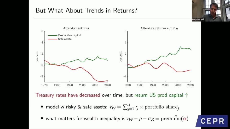
Is $\kappa > 1$ in the relevant population? That is measured, not assumed, and it is the nicest piece of empirical work in the paper. Building $\kappa$ from dina and the Fed’s distributional accounts for the top 1% by income and by net worth — and adjusting for the fact that the businesses investors own are themselves levered — gives values between 1 and 1.5, close to 1.3 in 1980 on the measures nearest the model. Investors top up each dollar of their own with about thirty cents of borrowing from other households. Not a knife-edge, not enormous. Meanwhile the safe rate fell about three points over 1960–2020 while three separate measures of the return to us business capital rose one to two points over 1970–2020, and the relevant gap — $r_W - \rho - \sigma g$, the object the tail index actually depends on — rose 1.5 to 3.5 points since the 1980s, partly because trend growth $g$ fell about 1.2 points along the way.

Then the caveats, all of which are the paper’s own. The right-hand panel omits $\rho$ entirely; the empirical $r_W$ omits the risk adjustment in equation (13); and the paper’s claim is that the growing return gap is a “potential driver” of observed inequality, not a measured contribution. Most importantly: this is not what the calibrated automation counterfactual produces. Feed the automation shock into the model and both returns rise — the safe rate from about 4.9% to 5.2% alongside risky capital from 6.5% to 7.0%, with the spread widening between them. Inside the model, automation pushes the safe rate up. The falling-safe-rate result is a comparative static, consistent with the measured 1960–2020 series where $r_B$ fell for reasons outside the model. Confusing the two would turn a careful conditional statement into a claim the paper never makes. The honest version is narrower and still useful: a falling safe rate is not evidence against this mechanism, and for levered investors it mechanically helps.

What Calvet did with it

Laurent Calvet of edhec — introduced by the chair, through asr or bad audio, as “Loic Calvez” — spent the first eighteen minutes of a twenty-eight-minute discussion rebuilding the model on his own slides in finance notation, which is both the highest compliment a discussant can pay and a useful compression: “this is a very beautiful and elegant model… it’s ingenious, it’s pedagogical.” He is right that the defining feature is the joint treatment: “there’s this disconnect often between the two aspects of income and wealth and it’s really good to be able to think about them jointly.” He also independently rederived the Pareto tail and reported having “had fun just checking the formulas,” which is roughly how an economist says a paper is correct.

Then five pushes, of which three landed.

The first is that the dissipation shock is alien to finance and under-explained where it matters — inside the household’s problem. “I would have liked to see a little bit more discussion of the interaction between $p$ and the optimization problem… from a finance perspective, slightly more explanations might be useful.” Fair, and it came back in the Q&A.

The second is a note that these are steady-state comparisons off a one-time unexpected shock, and “in an economy in which automation is a steady process, there might be more going on. People might want to hedge the automation risk.” Nobody answered this, and it is the kind of objection that is easy to state and expensive to address.

The third is his main one, and Moll conceded it outright. The equity return in the extended model is a Brownian motion bolted onto the asset, not derived from the production side: “my sense is that the Brownian motion was basically unrelated to what was happening in the production sector. You just tacked on a Brownian motion… Not sure what this represents. It doesn’t seem to be technological risk. Maybe it’s discount rate risk, I don’t know.” And the question a finance seminar always asks: “when there is a risk, is it priced? I’m not quite sure what the answer is — or maybe it’s not priced because it’s orthogonal to everything else.” He then showed how he would do it — shock the firm’s ebit, add a collateral-driven tax shield so debt scales with capital, value the equity, and read off a return that is tied to the shock that hit the firm — and noted that his setup delivers the same comparative static: a shock to automation raises the average return on capital and raises the capital stock too.

Moll’s answer was a clean concession. The Brownian motion “is indeed meant to capture idiosyncratic production risk. Basically, exactly like in your work with Marios [Angeletos]. But you’re correct that if that’s the case, because it’s a general equilibrium model, strictly speaking we should spell out where that shows up on the production side. We basically had some internal notes at some point where we spelled this out, and we convinced ourselves that you can sort of do it. But then we didn’t put it in the paper, which I guess makes it a little hard to follow.” The intended reading is entrepreneurs bearing uninsurable idiosyncratic risk; the general-equilibrium mapping exists, in a drawer.

The fourth push was the most generous thing in the session. Calvet took the paper’s own admitted failure — transition dynamics too slow — and offered the fix as a finished empirical fact. In his work with Bach and Sodini on Swedish administrative data, “we consider a very simple accumulation rule in which households just earn the historical portfolio returns and have homogeneous saving rates… if you just use the return that they earn on the assets that they had at the end of year $t$, then essentially you can predict very well the distribution of wealth in year $t$ plus one.” He showed predicted against observed annual changes in the top-1% and top-0.01% wealth shares. “If you know portfolio returns, you can basically figure out what the top share is. So this is very powerful.” Plus two regularities worth absorbing: returns rise with wealth, which Piketty conjectured and they document, and returns rise with age among the wealthy.

Moll did not defend: “I’m a huge fan of this literature. I 100% believe that’s super important.” The reason it is absent is tractability. What you would need is persistent types — some people always earning higher returns than others — “and that was just something that would have made the formulas less nice. But if you ask me, how can you fix this model? That’s exactly where I would go.”

The fifth push was the horse race. Calvet listed the competing stories — the entrepreneurial cost of capital, pension saving responses to low rates, tax progressivity, and a paper by Gomes, Jansson and Karabulut in which workers exposed to displacement risk rebalance away from stocks and therefore earn lower returns, amplifying the same inequality — and asked the obvious question while conceding it wasn’t this paper’s job: “do you think automation is a key channel? How does it compare?” Moll agreed a horse race would be a cool paper and then supplied the best available description of what this one is: “This paper is focusing on one particular mechanism, trying to really come up with a clean theory of how that works, and putting some suggestive numbers on this.”

Suggestive numbers. Hold onto that phrase; it is more accurate than anything in the abstract.

The Q&A, which produced the sharpest question of the session

Two questions in thirteen minutes. The first, from a participant the chair names only by a first name that the audio does not reliably deliver, opened with “I didn’t read the paper, so I probably missed exactly what’s going on” and then asked the best question anyone asked all afternoon, in two parts.

Part one: isn’t the return gap just a risk premium? “You have to put more of your money into savings because capital is more productive, and now you risk this displacement, and you’re risk averse, so you require a risk premium for that… then it’s kind of like fair return on the extra risk you take.” Part two, which is the sting: if the displacement shock is idiosyncratic and i.i.d. across people, “which is not how it works in finance either, right? Because then you should be able to diversify away this thing and you shouldn’t have that risk premium. And in fact we know that risk premia have kind of gone down over time.”

Moll said no, flatly, and the disavowal is worth having because it is not in the paper in this form: “I wouldn’t understand it as a risk premium. More like it’s a steady-state condition. So the way I think about it is it’s quite mechanical.” Everyone starts with zero financial wealth and returns to zero whenever they are wiped out, so the entire capital stock is the cross-sectional average of fortunes accumulated out of saved labour income. For that average to be positive against a wipe-out rate $p$, households have to be accumulating rather than sitting still, and that requires $r > \rho$. He tried to bring the wealth sawtooth back on screen — “there was this graph, maybe let me show it just briefly again. Um so, oops” — and narrated it from memory instead: “if $R$ were equal to rho, then that line wouldn’t be upward sloping, it would just be zero. And then everyone would just always stay at zero, and you wouldn’t have positive capital supply, and you wouldn’t have equilibrium in the capital market.”

That is the right answer and it also concedes something. The return gap is not compensation for anything; it is the amount of drift the accounting requires. Which is a slightly awkward thing to say about a wedge the paper then uses to explain who gets rich.

The diversification half was never squarely answered on the call. The paper’s answer is a footnote: the microfoundation in which dissipation is an extreme form of capital-income risk needs households to be unable to diversify across product lines and risk-sharing to be limited — “otherwise, an investment company could collect all investments and offer households a risk free return of $r - p$, which they would prefer.” Which is to say the objection is correct, and the model requires the frictions that defeat it.

When the questioner pressed on whether households at least internalise the shock, Moll said “100%,” and noted that under a Blanchard–Yaari reading with annuities the whole thing “basically just shows up like a higher effective discount rate and it doesn’t change anything else.” Then the methodological defence, which is the honest bottom line on the entire device: Aiyagari-class models have all the features you want, “the issue with that type of models is you can only solve them on a computer… And that comes at the cost of — yeah, there’s a little bit of a tension, like what exactly is this dissipation risk supposed to be?”

The second and final question was short and better than it looked: what would a declining relative price of investment goods do in this general equilibrium? It is, after all, one of the standard competing automation stories. Moll: aggregates would behave as in a standard neoclassical model, more capital accumulation. “What I haven’t thought about is what would happen to wealth inequality, which is I guess the interesting question. I don’t know off the top of my head.” And then, immediately and correctly: “what’s nice about this model is that you have everything with pencil and paper and you can just add that to the equations and then do the comparative statics… I’m pretty sure in that case you should still be able to solve everything in closed form. But I just haven’t done it.”

Which is a fair advertisement for what the paper actually bought with all those stark assumptions. The price of the dissipation shock is that nobody in the room, including the authors, is entirely sure what it is. The return on it is that when someone asks a question the model has never been pointed at, the answer is an afternoon’s algebra rather than a grant application.