Recent Developments in Current Employment Statistics

The Bureau of Labor Statistics turned up at a conference largely populated by people who complain about the payroll number and spent twenty minutes listing, in order, the four ways it can be wrong. Chris Manning and Steve Mance wrote the paper; Mance presented it, opening by noting that he is not Chris Manning, though the surnames are close enough that autocomplete occasionally routes him Manning’s email. The paper was commissioned for the conference, is unpublished, and carries the standard line that nothing in it constitutes bls policy — a disclaimer that is doing more work than usual, given what the paper concedes.

Start with what the number is, because almost everything follows from it. The Current Employment Statistics survey covers about 119,000 businesses and government agencies across roughly 622,000 worksites, reporting for the pay period containing the 12th. It does not count jobs. It estimates the change in jobs, recursively, by taking last month’s estimated level, stripping out the atypical self-representing units (influential reports, outliers, strikes), multiplying what remains by the ratio of weighted employment this month to last month among establishments that reported positive employment in both months, adding the atypical units back, and then adding a modelled birth–death term. On the slide it looks like this:

Here $\widehat{AE}_t$ is the estimated all-employee level, $ae^{T}_{i,t}$ is reported employment for matched sample unit $i$ with weight $w_i$, $ae^{A}_{j,t}$ is the atypical employment taken out and put back, and $b_t$ is the net birth–death adjustment. It is slide 6 of the presentation and it appears nowhere in the paper, which is a shame, because it is the whole argument. Notice what is missing: there is no non-response term. Non-respondents are not estimated, they are assigned — silently given the growth rate of whoever did respond in their estimating cell, usually a detailed naics code, sometimes crossed with Census region. That is missing completely at random within cell. Mance’s own gloss, delivered without visible discomfort: “a pretty strong assumption.” About a third of eventual responders arrive too late for the first print, so the first print is the one leaning hardest on it. And $b_t$ is the only term in the equation that is not data at all. It is a forecast.

Are the revisions actually misbehaving? The paper runs the Aruoba (2008) checklist — mean zero, small variance, unpredictable — and the answer is mostly no, with one large asterisk. From January 2003 to June 2026 the average initial-to-final revision is +7,000 seasonally adjusted, +8,000 not. The paper is honest that this is useless as a correction: the values “can diverge well from zero” and the mean is not a number you can subtract. Average absolute revision since 2005 is 51,000 seasonally adjusted, 53,000 not. The standard error of a one-month change in total nonfarm is 74,000 as of 2026. So the typical revision is meaningfully smaller than the sampling error of the thing being revised, which is a sentence worth sitting with the next time a revision leads the evening news. Revisions in 2023–2026 have been slightly larger than in the 2010s, but not above the post-2003 average.

The Wilcox puzzle. David Wilcox (2025) posed the awkward version: bls now receives vastly more information between the first and second estimates than it used to, yet the first revision is no more variable than it was two decades ago. If the gap between initial and final collection rates has blown out, why hasn’t the revision blown out with it? ces went looking and found that the collection rate has quietly stopped measuring what people think it measures. Both the collection-rate ratio and the ratio of weighted matched employment averaged around 80 percent through the 2010s, the weighted measure two to seven points higher. After 2020 they come apart: weighted matched employment stays above 80 percent every year, while the collection-rate ratio averages about 69 percent from January 2023 to June 2026.

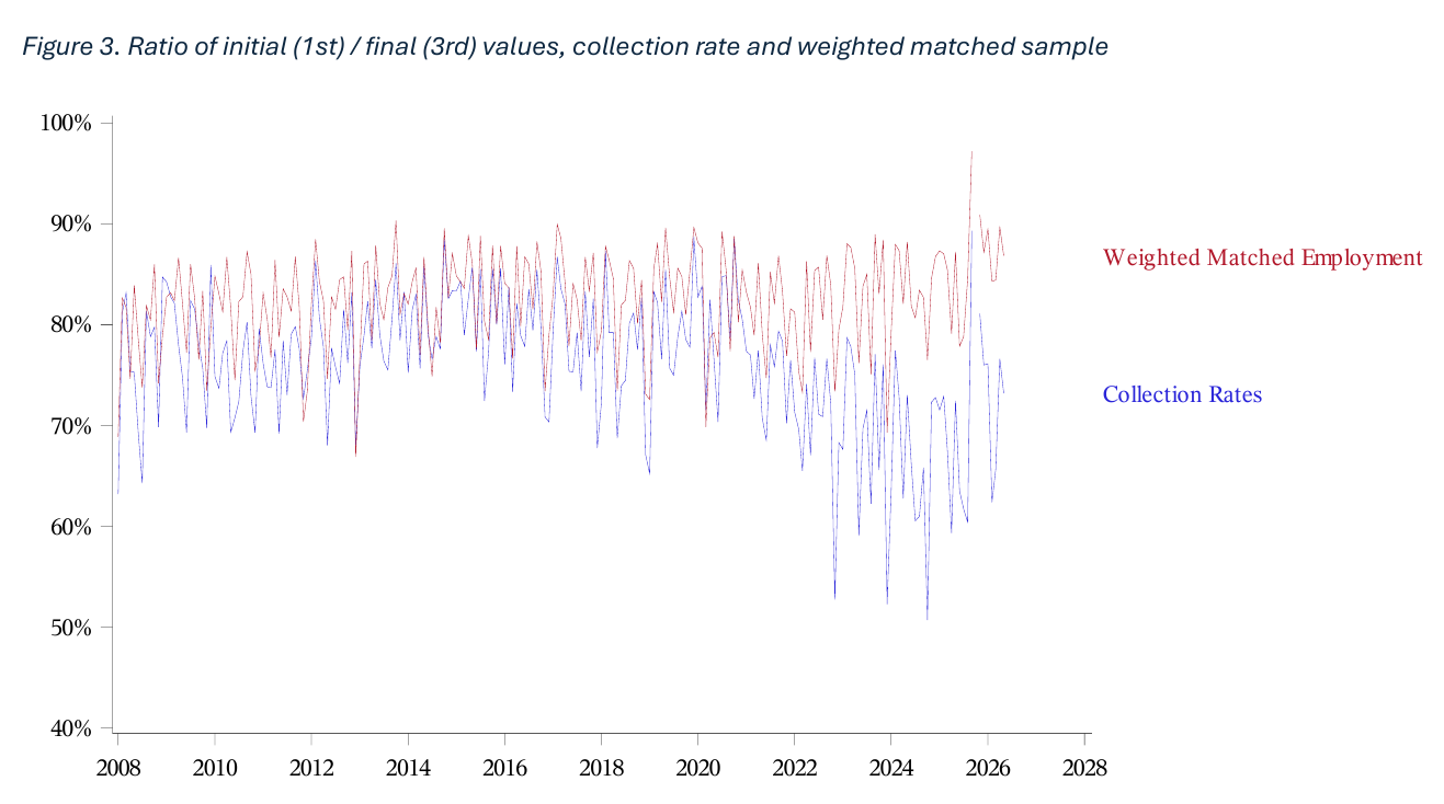
Which is to say the missing forms are increasingly small ones. “The late respondents are increasingly representing fewer weighted jobs per establishment,” as Mance put it. The monthly series behind that picture is in the appendix, and it does not drift: 97 percent in September 2025, 89 percent in January 2026, 90 percent in April 2026. October 2025 is blank, because the data “were not produced or published on their planned timeline due to a lapse in funding,” which is its own comment on the state of American economic measurement and is left, in the paper, entirely to a footnote.

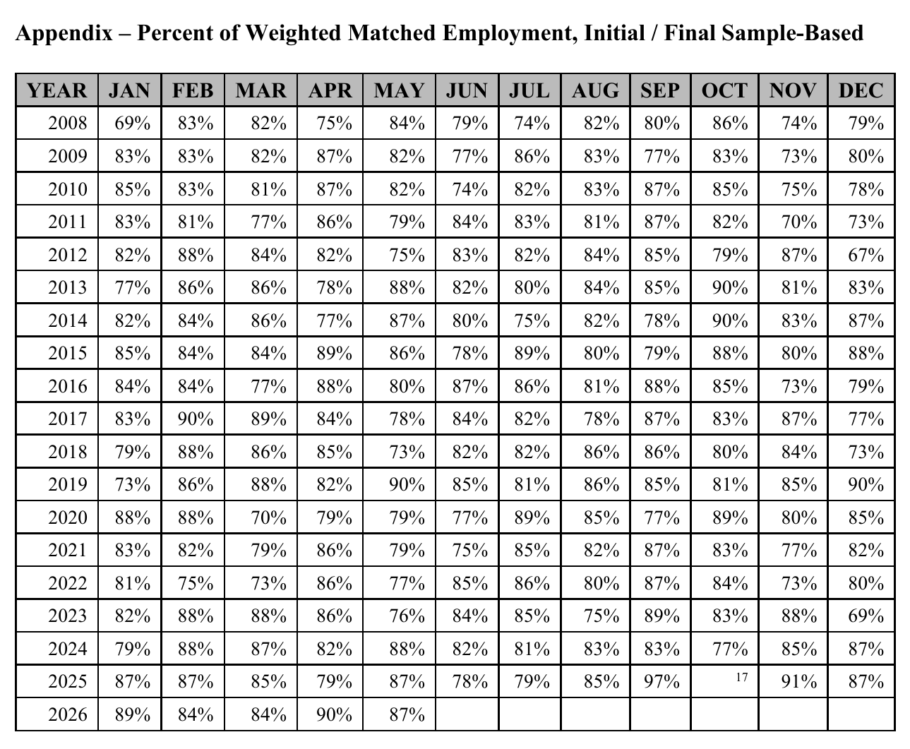
This is the cleanest answer available to the “the data are broken” critique, and it comes with a monthly table. It is also, as the paper does not quite say, an answer about information, not about bias. Nothing here rules out the possibility that the forms which fail to arrive are systematically the wrong forms. Hold that thought.

Now the part that should be better known. The paper’s sharpest exercise is one nobody asked for. ces ran seasonal adjustment repeatedly on employment series that were themselves never revised — January 2025 third closing as the endpoint, then February, then March — so that the only thing changing between vintages is how much future the seasonal filter has seen. The underlying data are frozen. Every month from February to November 2025 still revises downward from its concurrent value, and by the December run the seasonally adjusted levels for June, August and September 2025 were each over 90,000 lower than where they started.

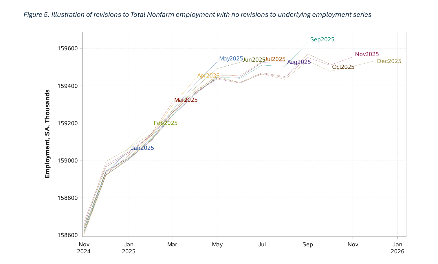
The mechanism is not mysterious once stated. Concurrent seasonal adjustment extends each series with a RegARIMA forecast before running the X11 filters, because the alternative is badly asymmetric end-of-series filters that everyone agrees are worse. So the seasonally adjusted number embeds a forecast of the next month or two, and in a year when growth decelerates, that forecast is wrong in a consistent direction, and the correction arrives as a revision. The paper is candid about the residue: across the 148 series ces adjusts directly, the aggregate one-step-ahead forecast errors show serial correlation and are not centred on zero, which is an invitation to intercept corrections in the style of Castle, Doornik and Hendry. Research on the forecast extension starts in 2027 — “this next fiscal year that starts in about a week or two,” Mance said. There is also a splice: the third-closing over-the-month change compares two vintages of seasonal factors, since only the prior two months are updated. The slide cites Wright (2013) recommending that the entire series be re-adjusted every month instead. That recommendation does not appear in the paper text, and it amounts to a bls slide conceding that the two-month window is a publication convention rather than a statistical decision.

The implication is uncomfortable for a popular critique. When commentators point to the cyclicality of revisions as evidence that the survey is degrading, a large share of that cyclicality is the seasonal filter forecasting into a turning point. The 2021 numbers make the point arithmetically: +159,000 average revision seasonally adjusted, +59,000 not seasonally adjusted. Two-thirds of the famous 2021 upward revision came from the adjustment, not from late data. The slide says it flatly — without revisions to the unadjusted data, seasonally adjusted revisions would have been consistently negative in 2025.

The blind spot you cannot survey your way out of. A new business reaches the ces sampling frame seven to nine months after the reference month, and in practice it takes at least a year to sample, contact and verify. Closures are symmetric: a business that has shut down is not prioritising its ces form. So “actual” birth–death is constructed as the amount you would have had to add to a ces-style estimate run over the qcew universe if births and deaths were never observed in real time — and then that constructed series is forecast, and the forecast is $b_t$. Cumulatively it is enormous: total private job growth of roughly 24 million from March 2013 to July 2026 against actual birth–death near 12.5 million. Month to month, Mance was careful to say, “it matters, but it’s far less important than change from continuing establishments.”

The old forecast was a seasonal arima that assumed birth–death reverts to its own seasonal history, and was, in Mance’s words, “not at all responsive to turning points” — a deficiency the pandemic exposed at maximum volume. The replacement conditions a RegARIMA on the current sample link relative, which is to say on the middle term of the estimator above: the survey forecasting its own blind spot off the one thing it does observe.

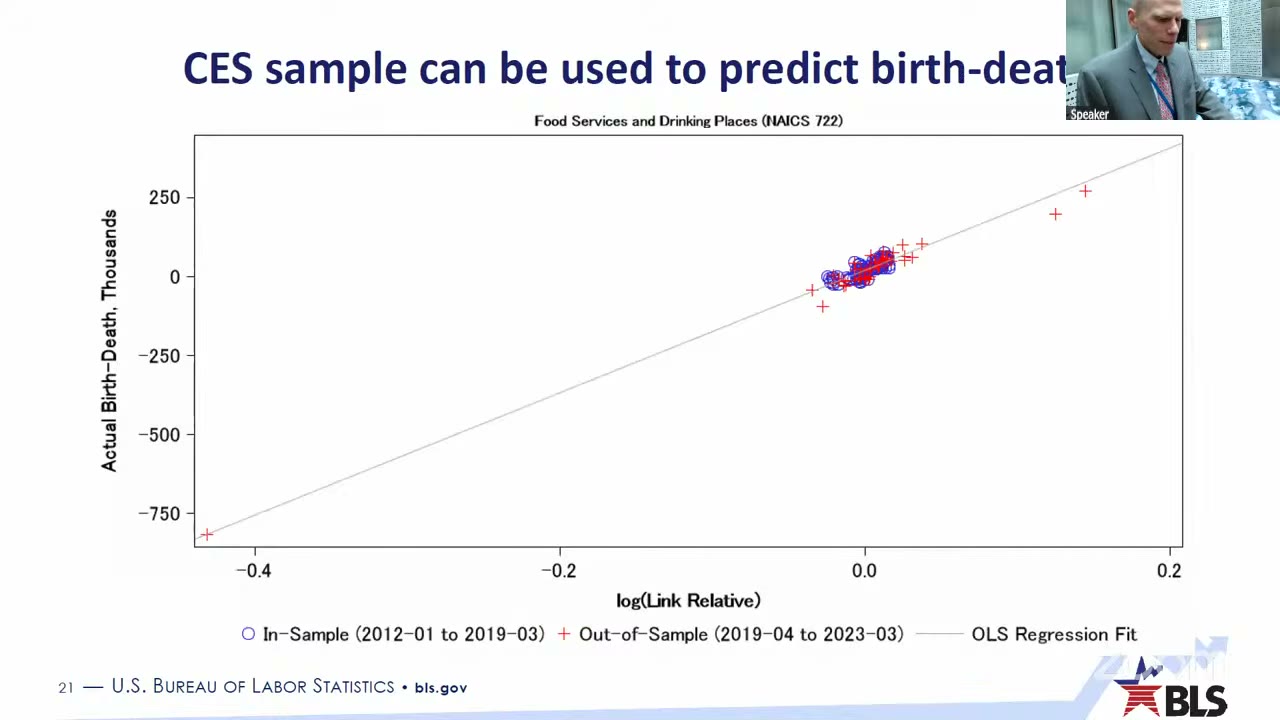
It went into production for the April–October 2024 post-benchmark re-estimates and has run monthly since the January 2026 estimates, and Mance’s claim for it is specific: the March 2025 benchmark revision, which was large and much discussed, “would have been substantially larger had we not done this.”

The discussion, which supplied the objection the paper does not make. John Haltiwanger had both Session 1 papers and declined to re-summarise either, calling them outstanding and the underlying expertise “just enormous.” Then he pushed, four times. Make the benchmark quarterly: the qcew could support it, market participants and bea already use the quarterly releases to predict the annual benchmark, and the reasons bls gives — first-quarter data are better than the other three, benchmarking is expensive — are resource constraints rather than statistical ones. “A priority ought to be put on this.” No author answered this, and the floor never came back to it. Modernise the pipeline out of legacy sas and into Python so administrative data can be processed faster, because payroll and ui tax data exist well before they surface in the qcew or the business register, and there may be signal in an early read. On birth–death, a warning aimed at the whole alternative-data enthusiasm: “The payroll data doesn’t help you really at all on this.” You need a high-frequency external indicator — the Census Business Formation Statistics, weekly and near real-time, on which he declared his own co-authorship, or ui claims, which are “sitting there.”

And then the one that lands on the equation. “This idea that there’s inside cells, there’s missing at random, is just wrong. I think we already know that.” He has evidence: work with Steve Davis, Jason Faberman and Ian Rucker matching micro jolts to the bls longitudinal database inside bls, with qcew as truth. The finding is not the one ces already builds around. It is not only that closing businesses fail to report — “businesses that are contracting rapidly aren’t filing reports.” Put that next to the matched-sample ratio and the problem is immediate: every non-reporter gets assigned the growth of the firms that did report, the non-reporters are disproportionately the ones shrinking, and the bias therefore runs in the direction of overstating employment exactly when employment is falling, and worsens as response rates fall. Overall ces response rates have stabilised in the low 40s. Haltiwanger’s point about payroll data is the same point from the other side: “maybe you don’t respond to the bls survey, but you’re still making your payroll.”

To the authors’ credit, the composition finding is not a defence against this, and they did not use it as one. Their one substantive turn from the floor — on degraded audio, so read with care — conceded the structure of the charge directly: when non-response “is related to what we’re trying to measure, then really the problem is” there, and the strategy is to find observables to adjust on. They are doing exactly that, with multiple imputation and tree-based weight calibration by state and size class under test, and a contracted non-response bias analysis due to be public by the end of 2026. The most charming version is the industry-specific fix: in sports teams, one April, baseball clubs responded far more than hockey and basketball clubs, which is to say the hiring ones reported and the laying-off ones did not, and a sport dummy would have caught it. They also confirmed they had looked at Haltiwanger’s birth–death suggestion back in 2013 and “it worked okay,” but tied the latest round to ces sample data deliberately, and they are exploring linked administrative counts — if a non-responding business is laying off a lot of people, “that probably tells us something about what’s happening there.”

What ces can already show on predictability is narrow and honest. Out-of-sample over 2016–2025, an ar(3) beat a zero baseline on seasonally adjusted total nonfarm only slightly, with the gain concentrated in 2021 and not significant. Across 100 industries, mostly three-digit naics, exactly one shows clear predictability in published revisions: Local Government Education, running above +50,000 for several Augusts in a row. A RegARIMA on historical school-district growth plus the already-reported first-closing sample would have cut the average August absolute revision from 62,000 to 29,000 over 2015–2024, still positive, still “continued room for improvement.” That now-cast goes to ces analysts as advisory, not automatic, and has since August 2025. The quieter result is the one that should reassure: several industries look predictable in counterfactual revisions computed as if ces had never made its existing certainty-unit imputations, and none look predictable with those imputations in place. The manual work is already doing the job. For private-sector late sample, many approaches beat the implicit imputation at the micro level and none yet improves macro revisions — the same wall Copeland and Valliant hit in 2007.

The floor then changed the subject to survival. David Wilcox said the thing nobody had said, which was that the whole adp discussion was in the past tense, because adp no longer supplies those data to the Federal Reserve Board. “The Federal Reserve Board effort was a live ammunition exercise. We were putting this information in front of the open market committee and allowing them to make policy decisions because we decided that the product, the blended product, was high enough quality to warrant that, and suddenly it was cut off. What happens if?” Michael Stepner then flipped the framing entirely: rather than making do with the qcew as the benchmark for private data, improve the administrative data the government collects by requirement — the uk reformed payroll reporting so firms report to government more frequently. Matthew Shapiro, on organisers’ privilege, tied the two together: ad hoc contractual feeds can be cut off; an infrastructure where payroll data flow once and are routed both to the states for benefits processing and to bls for statistics cannot.

Which leaves the bls paper in a slightly odd position. It is a genuinely good audit — the freeze-the-data seasonal adjustment exercise is the kind of thing an agency does only when it wants to know, and the answer it produced is embarrassing in a useful way. It resolves the collection-rate puzzle with a measure nobody had constructed. It fixed birth–death by noticing the forecast it needed was sitting inside its own estimator. And the one assumption it flagged as strong and then kept — missing completely at random inside the cell — is the one its discussant says is demonstrably false in the specific direction that matters, on evidence collected inside the same building. Everyone in the room agreed that the fix, whatever it turns out to be, runs through better benchmark data. The appendix to this very paper already contains one month in which the data were simply not produced, because the money stopped.