The Macroeconomics of Supply Chain Disruptions

Daron Acemoglu (MIT) and Alireza Tahbaz-Salehi (Northwestern, Kellogg), “The Macroeconomics of Supply Chain Disruptions,” Review of Economic Studies 92(2), 2025, pp. 656–695 (advance access 10 April 2024). The earlier version is NBER Working Paper 27565 (2020), under the blunter title “Firms, Failures, and Fluctuations.” The talk is Tahbaz-Salehi’s 27-minute presentation at the NBER Economics of Supply Chains meeting, 26 January 2024, organised by Laura Alfaro and Chad Syverson; there was no discussant, and the “Chad” the speaker turns to for a time check is Syverson. The two images below are both crops from the published version — Figure 3, the two supply chain architectures, and Figure 4, the fragility comparison. No slide from the talk is reproduced.

A supply chain link is a public good that nobody is paid to provide

Start with one relationship. You are a firm — call yourself $j$ — and you can sell a customized input to firm $i$. Customizing costs you a fixed sum $s$: retooling, joint R&D, redesigning your part so it fits their product. The cost is relationship-specific, which is the technical way of saying that if the relationship ends, the money is gone and cannot be carried to the next customer. In exchange, the two of you are jointly more productive than either would be alone. This is the Adam Smith story the speaker opens with, and the running example is Airbus, which claims 12,000 suppliers and does not build its own engines because GE and Rolls-Royce build better ones — provided the engine is designed to fit that airframe, which is the relationship-specific part.

Now ask the only question that matters: who gets the extra output? Not you, or not all of it. You bargain with $i$ over the split. But $i$ has customers who are more productive because $i$ is more productive, and they bargain with their customers on terms that reflect how much surplus is floating around, and so on down the chain. Your fixed cost quietly improves the bargaining position of firms you have never met, and none of them send you a cheque. You pay for the link; the chain eats the returns.

That is the entire paper. Everything else is the machinery for saying it precisely and then following it somewhere unpleasant.

The model, which is a bargaining game wearing a production network as a disguise

There are $n$ input producers and a final-good firm indexed 0. Each firm has a menu of constant-returns technologies, indexed by which set of inputs it uses, with a productivity $A_i(I_i)$ attached to each input mix — Airbus with a GE engine and Airbus with a Rolls-Royce engine are two different technologies, not one technology with a substitutable part. Using a designated supplier’s customized input requires both sides to sink a fixed cost: $c_{ij}$ paid by the customer, $s_{ij}$ paid by the supplier. Pay them both and the link exists; the collection of links is the production network.

Prices are then set by pairwise Nash bargaining over two-part tariffs — a per-unit price plus a lump-sum transfer — with bargaining weights $\theta_i$. Two details do a lot of work. The two-part tariff means the pair sets the unit price to maximise their joint surplus, which is marginal cost, and does all the fighting over the lump sum; so there are no markups and the transfers are purely redistributive. And the contracts are network-contingent: if you and a supplier fail to agree, everyone else’s contracts are renegotiated in the smaller network. That is Stole–Zwiebel, and the paper is explicit that it is not Nash-in-Nash, where the rest of the chain’s prices would be frozen during your disagreement. Network-contingency plus two-part tariffs is exactly what makes the fixed-network equilibrium efficient, which is what lets the authors pin every inefficiency in the model on the extensive margin.

With the network held fixed, an equilibrium exists, is generically unique, and is efficient, and Theorem 1(c) gives each firm’s gross profit in closed form:

which is equations (6) and (7). Force the notation to say what it means and it is friendly: your profit is a weighted average of your marginal contribution to aggregate productivity, taken across every subnetwork you could belong to, with the weights set by everyone’s bargaining powers. The authors note this is the weighted Myerson value, the network-adjusted generalization of the Shapley value. Contribute nothing to aggregate productivity and you earn nothing; have no bargaining power and you earn nothing. It is a cooperative game hiding inside a general equilibrium model, and it is why the surplus you create leaks to strangers — the Myerson value shares your marginal contribution around and never asks who paid the fixed cost.

The comparative statics run through two supermodularity conditions — an extra link is worth more in a larger network (extensive margin), and worth more when the existing relationships are more productive (intensive margin). Given those, expanding the network or improving any link raises every firm’s profit, and raising one firm’s bargaining weight raises its profit and lowers everyone else’s. Theorem 8 is the productivity version, and its stated implication is that supply chains are procyclical: firms build relationships in good times and shed them when productivity falls, which the authors match to Xu et al. (2023) on the procyclicality of the US supplier count.

Under-investment, and why under-investment produces cliffs

Turn the network endogenous. An equilibrium exists, there is a greatest one that contains all the others and Pareto-dominates them, and it is a strict subnetwork of the efficient one. Tahbaz-Salehi was careful in the talk to say there are two externalities pulling opposite ways. Adding a link expands the production possibility frontier and the gain is shared with everyone, which the pair paying for it cannot appropriate — under-investment. Adding a link also improves the pair’s bargaining position at everyone else’s expense, which the paper calls the surplus-redistribution externality and the talk called business-stealing — over-investment. Supermodularity is precisely the assumption that the first dominates. So firms build too few relationships.

The payoff is Theorem 10. Efficient aggregate output is continuous in productivities and fixed costs; equilibrium output is generically discontinuous, and discontinuous exactly where the equilibrium network changes. The intuition is the one-link example: raise the fixed cost $s$ on a single relationship and the planner keeps paying, so efficient output slides down smoothly until the link stops being worth it and then goes flat. The firm bearing the cost quits earlier, because it never counted the surplus its link creates for others. At that earlier point output falls off a step to the floor the planner would only have reached later, and the height of the step is the distance between the two indifference points. Inefficiency and fragility are, as both the paper and the talk put it, two sides of the same coin — the cliff is the wedge, measured vertically.

The efficient supply chain is the one that goes first

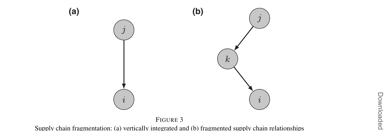
Here is the application, and it is the one that matters for this reading list. Compare a vertically integrated chain, where $j$ supplies $i$ directly, with a fragmented one, where $j$ supplies a specialist $k$ who processes the input and passes it to $i$. The comparison is built so that the only difference is the fragmentation. The rest of the network is held fixed, the $i$–$k$ link is free, and $j$ pays the same fixed cost $s$ either way, whether its customer is $i$ or $k$. Both architectures contain exactly one costly link. Then assume, as equation (13) does, that

The first inequality is the specialization gain that motivates outsourcing in the first place. The equality on the right says $k$ is good for nothing except processing $j$’s output: without $j$, the specialist adds no productivity at all.

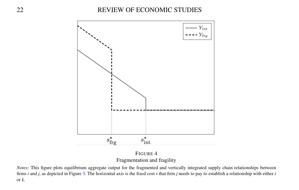
So why is Proposition 1 true — why can the fragmented chain break first? Not because it has more links to lose; it does not. It is because the fragmented chain has more mouths. In the integrated architecture, the surplus that $j$’s fixed cost creates is bargained over with $i$. In the fragmented one, that same surplus must now also pass through $k$, and $k$ arrives with bargaining power $\theta_k$. Proposition 1 is stated “for large enough values of $\theta_k$,” and that condition is the mechanism, not a technicality: when the specialist can extract a large enough share of the relationship surplus, what is left for $j$ no longer covers $j$’s fixed cost, at a value of $s$ where $j$ would still have been happy to supply $i$ directly. The paper’s own sentence is that “when firm $k$ can extract a large enough share of the surplus, the threshold of discontinuity in the fragmented architecture can be to the left of the threshold in the integrated architecture.” So the fragmented economy is more productive at every $s$ below its cliff, and it hits the cliff at $s^*_{\text{frg}} < s^*_{\text{int}}$, and because both economies land on the same floor — equation (13)’s right-hand equality guarantees it, since a specialist with nothing to process is worth nothing — the drop is larger as well as earlier. That is what “a sharper and an earlier drop” means, and it is what the crossing curves in Figure 4 are showing.

Two honest caveats. The result is a possibility, not an inevitability: the threshold ordering can reverse, for large enough $\theta_k$, and the paper says “can” both times. And the extra fragility is coming from the division of surplus, not from the length of the chain as such — a specialist with no bargaining power would not do this.

Cascades, and why the shock size matters more than the shock

The other two applications follow the same logic. In a vertical chain of depth $n$ with a common fixed cost $s$, Proposition 2 gives you the starkest version available:

which is to say the chain is either fully assembled or entirely gone. Push $s$ a hair past the point where the most upstream firm breaks even and it severs; that severance lowers aggregate productivity, which makes the next firm’s relationship unprofitable, and the collapse walks downstream. The footnote is careful to establish that this is a genuine cascade rather than a simultaneous shock: firm $n-1$ was making money and stops only because $n$ quit. And the size of the discontinuity grows without bound in the depth of the chain, which is a slightly alarming thing to have proved about an economy whose chains keep getting deeper.

Proposition 3 supplies the nonlinearity. Relationships break in order of productivity, cheapest first, along a decreasing sequence of thresholds $a_1 \ge \cdots \ge a_n$, so a mild downturn dissolves links that were barely worth having and costs almost nothing, while a severe one reaches into the productive relationships and costs a great deal. The supply-chain channel is a weak amplifier of ordinary recessions and a strong amplifier of the 2007–8 financial crisis or the COVID pandemic, which are the authors’ two examples — and the observed cleansing of low-productivity suppliers in normal recessions is therefore no evidence against catastrophic supply-chain effects in abnormal ones.

Where it sits

This is the theory behind the knife-edge language in the second Claude list and the formal reason the gotchas in block 1.0 exist. Baqaee–Farhi tell you networks amplify large shocks when the linkages are fixed — or, in the 2021 version with endogenous entry, that firms are infinitesimal and the mass of entrants and the number of links adjust smoothly, so nothing ever jumps. This paper tells you the linkages themselves give way, discontinuously, at the wrong point, and that the more finely divided chain is the one that goes first.

The comparison with Elliott, Golub and Leduc (2022) is the one worth getting right, because they are shelved next to each other and the results look alike. Their discontinuous phase transitions come from the technology — multiple essential inputs produced over infinitely many stages, so the chain works only if some undisrupted path continues upstream forever — and a discontinuity that lives in the technology shows up in the planner’s solution too. Here it does not. Theorem 10(a) says the efficient allocation is continuous in every shock, no matter how deep or complex the network. Fragility in this model is one hundred per cent an equilibrium artifact: it exists because decentralized firms sever links at their own indifference points rather than at society’s, and for no other reason. That is a stronger and stranger claim than “supply chains are fragile.” It says the cliff is not a property of the supply chain at all. It is a property of who is paying for it.

For geoeconomics the uses are two. The hegemon threatening to cut off an input is threatening to push a chain past its $s^*$, and the model tells you the threat is credible in a specific way — the loss is discontinuous, and it lands earlier than any planner would have chosen. And a country’s “economic security” policy is in part a decision about where to sit on the integrated-versus-fragmented trade-off, which Grossman, Helpman and Lhuillier turn into an explicit policy problem. Though on this model the honest version of the policy is less “build resilience” than “buy back the surplus that firms are giving away for free,” which is a harder thing to put in a strategy document.