Notes on:

Land-Price Dynamics and Macroeconomic Fluctuations

Zheng Liu, Pengfei Wang & Tao Zha
Econometrica
1 May 2013
land prices · collateral constraints · DSGE · business investment · housing · Bayesian estimation
Paper · doi · PDF
Fable 5 (reading), GPT 6-Astra (verification), Opus 5 (diagram and writing)

Zheng Liu, Pengfei Wang and Tao Zha, “Land-Price Dynamics and Macroeconomic Fluctuations,” Econometrica 81(3), May 2013, pp. 1147–1184 — read in the published Econometrica version. There was no talk, so there is no discussant and no Q&A; the objections at the end are a reader’s, not a room’s.

A credit line with a building on it. You run a mid-sized manufacturer and you would like to buy a machine. Your bank is not, in the first instance, lending against the machine’s future cash flow; it is lending against something it can seize and sell if you stop paying. Nearly 70% of U.S. commercial and industrial loans are secured by collateral, and the collateral is mostly dirt: in the Flow of Funds, tangible assets average about two-thirds of total corporate assets over 1952–2010 and real estate about 58% of those tangibles, while for nonfarm noncorporate firms real estate runs about 90% of tangible assets, which are in turn about 87% of everything they own. Chaney, Sraer and Thesmar find that over 1993–2007 a dollar more of real estate value bought a representative U.S. firm about six cents more investment, and more where the firm looked credit constrained; Gan finds that in post-bubble Japan every 10% fall in collateral value cut a representative firm’s investment by about 0.8%.

So the parcel under your plant is doing two jobs, and the smaller of the two is production — in this paper’s estimated production function the output elasticity of land is roughly two percent. It is mainly a borrowing base that happens to have a factory on it, which makes the price of land, mechanically, the size of your credit line. That is the whole paper.

The fact it wants explained is that land prices and business investment move together, and not just in 2008. A four-variable Bayesian VAR with the land price ordered first, fitted 1975–2010, says a positive land-price shock raises the land price, consumption, investment and hours, all persistently.

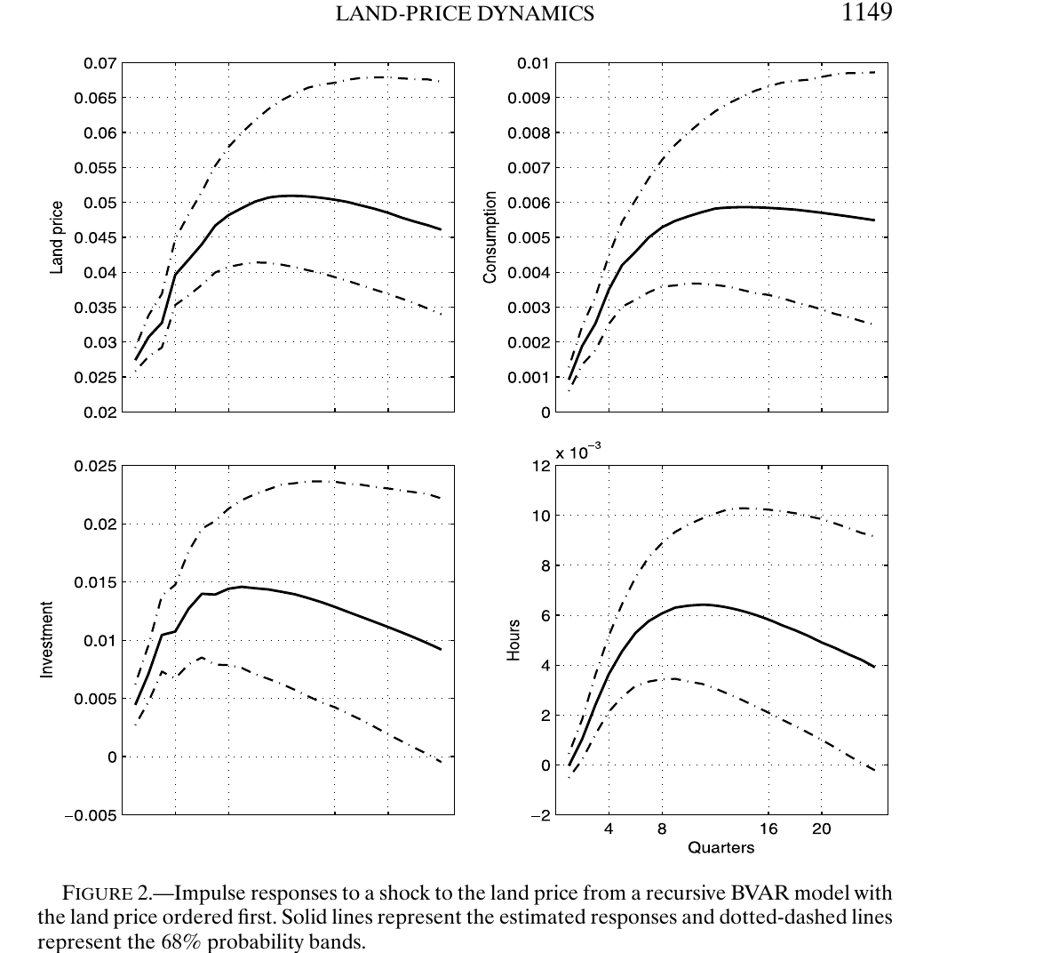
Four-panel BVAR impulse responses: land price, consumption, investment and hours all rise persistently after a positive land-price shock; the land price’s own response is the largest, and investment responds most among the three macro variables — Figure 2, paper p. 1149: impulse responses to a land-price shock from a recursive BVAR (land price ordered first), 1975–2010; solid lines are point estimates, dotted-dashed lines the 68% bands — the co-movement fact the model is built to explain.

This is more awkward than it looks. The existing DSGE literature on house prices — Iacoviello, Iacoviello and Neri — constrains households, who borrow against their houses to consume, and so gets house prices co-moving with consumption while struggling to get them co-moving with business investment. In a frictionless real business cycle model with housing the sign is flatly wrong: land is a fixed factor, so a household that suddenly wants more of it bids it away from firms and investment falls. The co-movement in the data is the thing standard theory says should not happen.

The model.

Land collateral and the competing demand for land. A schematic drawn for this digest — not an exhibit from the paper — showing the two agents, the two markets, the collateral gate on the credit edge, and the loop that runs from the land price through borrowing to investment and back. The frictionless benchmark, noted at the foot, is the same picture with the gate removed and the loop severed. Open the figure in a new tab

Two agents. A patient household that consumes, houses itself on $L_{ht}$ units of land, works and lends. An impatient entrepreneur who produces with land, capital and hired labour, invests and borrows. They meet in two markets: land, in fixed aggregate supply, so $L_{ht} + L_{et} = \bar{L}$ and two demands must be settled by one price; and one-period credit, where the friction sits. Contracts being costly to enforce, a defaulting entrepreneur can be stripped of his land and capital but the creditor recovers only a fraction $\theta_t$ of their value, so

B_t \le \theta_t \mathrm{E}_t\left[q_{l,t+1} L_{et} + q_{k,t+1} K_t\right]

which is equation (14): borrowing $B_t$ capped by a fraction $\theta_t$ (calibrated to 0.75 in steady state, and itself shocked) of the expected next-period value of the entrepreneur’s land at price $q_{l}$ and capital at shadow price $q_{k}$ . The household is estimated to be slightly more patient than the entrepreneur, which is what keeps this thing binding rather than slack.

Now write down what a unit of land is worth to each of them. To the household it is the discounted resale value plus the marginal utility of the housing services it throws off. To the entrepreneur, equation (21) with habit switched off for exposition,

q_{lt} = \beta \mathrm{E}_t \frac{C_{et}}{C_{e,t+1}}\left[\alpha\phi \frac{Y_{t+1}}{L_{et}} + q_{l,t+1}\right] + \frac{\mu_{bt}}{\mu_{et}}\,\theta_t \mathrm{E}_t\, q_{l,t+1}

where the first bracket is the future marginal product of land plus resale value and the last term is a collateral premium: $\mu_{bt}/\mu_{et}$ is the shadow value of a loan, strictly positive precisely when the constraint binds. That last term is the entrance to the loop. Land is worth more to a constrained firm than its marginal product, because owning it is how you get money.

The loop. Give the household a taste shock $\varphi_t$ — it wants more housing. Its land demand shifts up and the price rises, which in the frictionless world would be the end of it. Here the higher price mechanically enlarges the entrepreneur’s borrowing capacity, so his land demand shifts up too, the two of them compete for a stock that cannot grow, and the price rises again. That is the static multiplier. Then the dynamic one: more credit means more investment now, more capital next period, and because capital and land are complements in production, a higher future marginal product of land — which raises the land price today, which relaxes the constraint further. The paper draws it as a five-step walk.

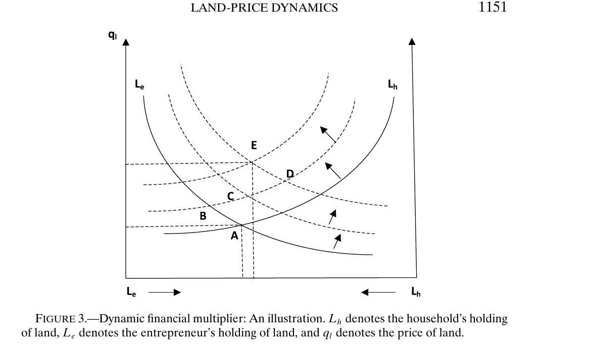
Supply-and-demand diagram in land-price/land-quantity space: household and entrepreneur land demand curves shift up in steps A to B to C to D to E, tracing the static and dynamic financial multipliers — Figure 3, paper p. 1151: the dynamic financial multiplier. A housing demand shock moves the equilibrium from A to B; collateral-fueled competing demand for land takes it to C, the investment-capital-land-price feedback to D, and the household wealth effect to E.

Here is the surprising part, and it is worth slowing down for. The force that was supposed to kill the result is the one doing the work. “Households outbid firms for land” is crowding out; it is why the frictionless model gets the wrong sign. But against a fixed supply, competing demand unambiguously raises the price, and price is what the constraint is written on. The paper’s comparative static is that the less land actually changes hands, the larger the land-price response. And in the estimated model the entrepreneur — the agent who was supposed to be outbid — ends up holding moderately more land, an increase of a bit under 3% of the total stock. The crowding-out channel got repriced as an amplifier.

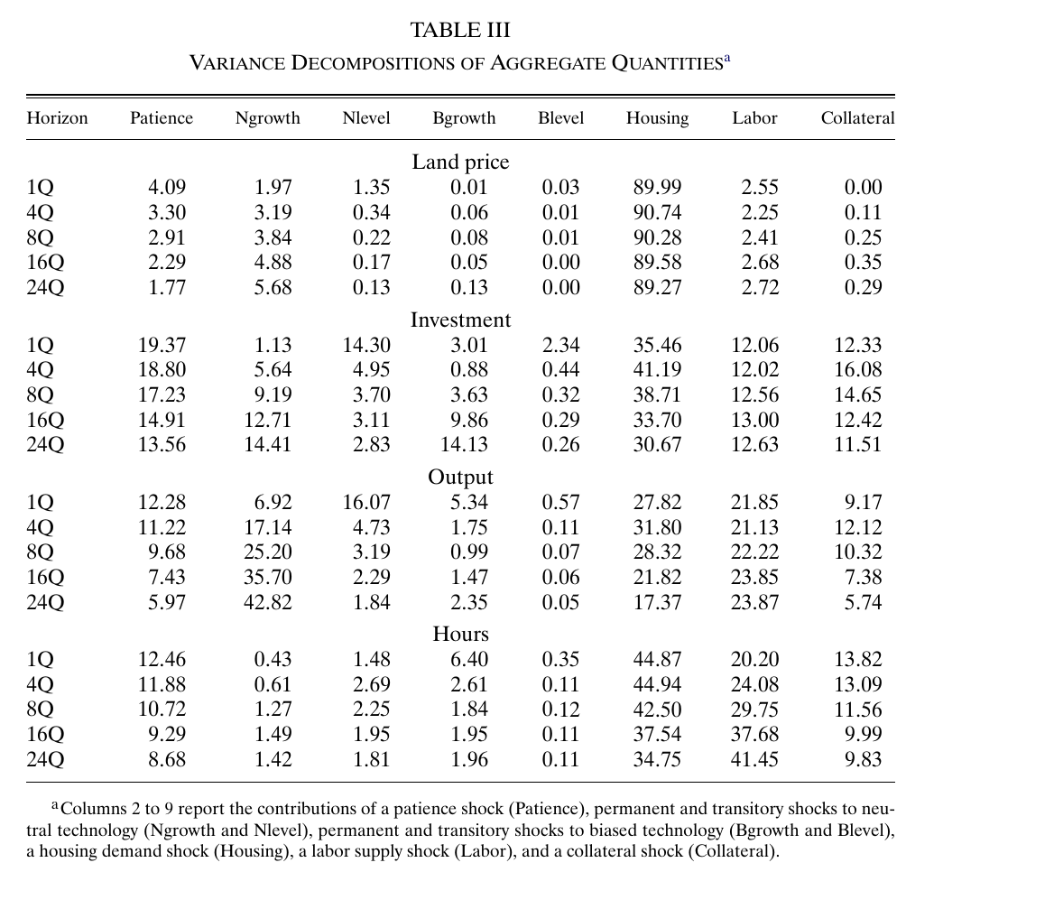
Why it has to be a taste shock. Fit the model to six quarterly U.S. series over 1975:Q1–2010:Q4 with eight shocks and you get a clean, slightly uncomfortable answer to what moves land prices. The land Euler equation makes the price a discounted sum of future marginal rates of substitution between land and consumption. Hold $\varphi_t$ fixed and that MRS is only as volatile as consumption — and land prices in the data are far more volatile than consumption. So TFP, investment-specific technology, labour supply and patience shocks cannot manufacture the observed land-price volatility; only a shock that enters the MRS directly can. The estimates duly hand the housing demand shock about 90% of land-price variance at every horizon and, through the collateral channel, 31–41% of investment, 17–32% of output and 35–45% of hours. (The paper’s prose says the other shocks “do not move land prices,” which is exactly true only in its linear-utility illustration; in the estimated model the runners-up are small but not zero, patience at 4.09% on impact and permanent TFP at 5.68% by 24 quarters. Dominant, not solitary.)

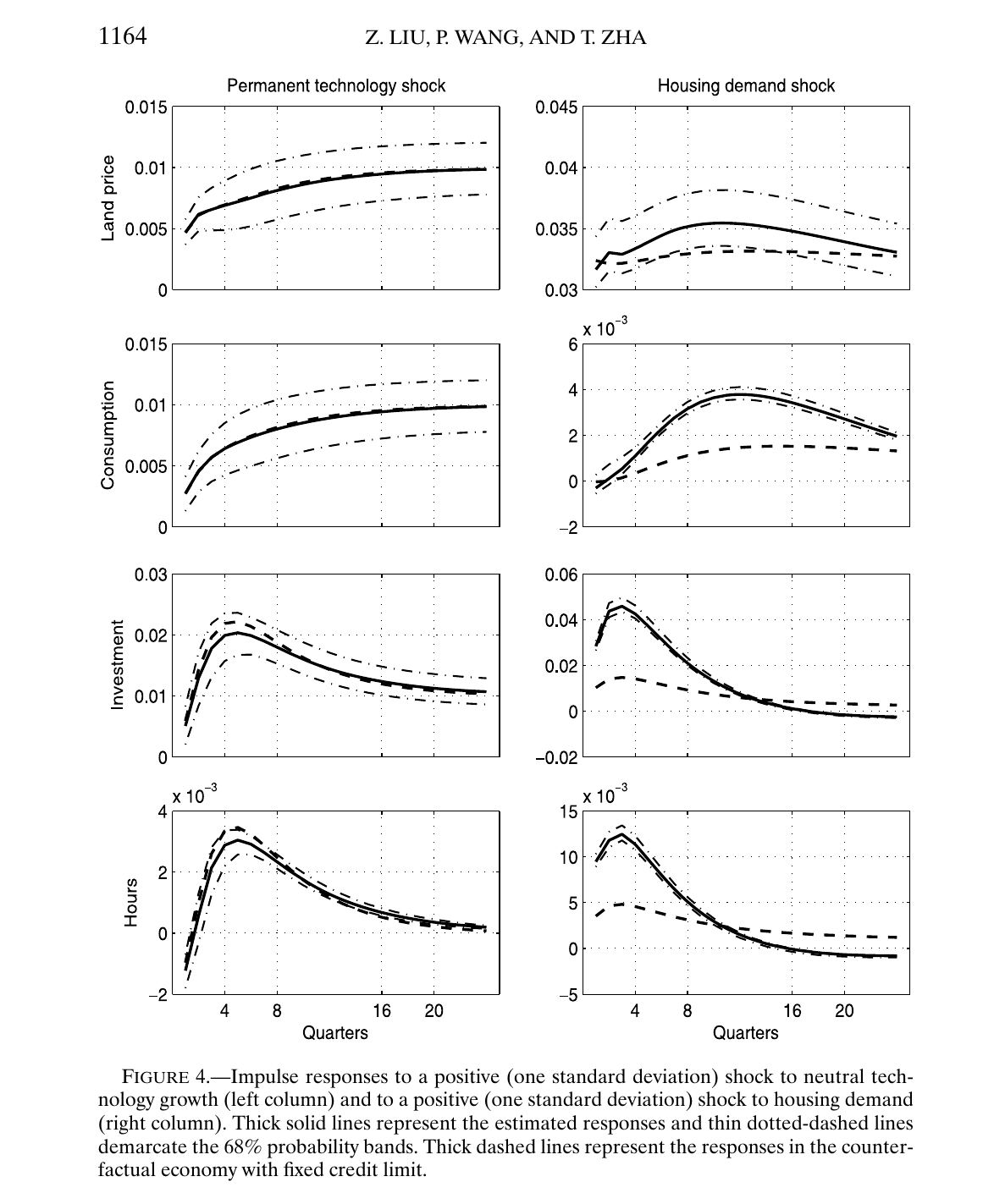
Variance decomposition table: the housing demand shock accounts for about 90 percent of land-price variance at every horizon, 31-41 percent of investment, 17-32 percent of output and 35-45 percent of hours — Table III, paper p. 1159: variance decompositions across the eight shocks. Housing demand owns the land price (~90%) and, through the collateral channel, large shares of investment, output and hours; no other shock reaches 6% of land-price variance.

Does the constraint actually amplify anything, or is it decoration? Re-run the model with the credit limit frozen exogenously and compare. To a TFP shock, almost nothing changes — the counterfactual sits well inside the benchmark’s 68% bands, which is the old Kocherlakota and Cordoba–Ripoll finding that collateral constraints amplify weakly, and which the paper explains rather than disputes: a TFP shock does not lift land prices, so there is nothing for the constraint to bite on. To a housing demand shock the two economies come apart, consumption, investment and hours responding several times more strongly once the credit limit is allowed to move with the land price.

Eight-panel impulse response comparison: for a technology shock the benchmark and fixed-credit-limit responses nearly coincide, overlapping fully for land price and consumption and separating only slightly at the investment and hours peaks; for a housing demand shock the benchmark responses of consumption, investment and hours are several times larger — Figure 4, paper p. 1164: benchmark (solid) vs. fixed-credit-limit counterfactual (thick dashed) responses. To a TFP shock the two are “not much different” — the counterfactual sits inside the benchmark 68% bands, so credit constraints barely amplify it — while they strongly amplify a housing demand shock: the amplification evidence in one picture.

Then the obvious test. Between 2007:Q3 and 2009:Q2 the real land price fell 25% and business investment fell 22%. Feed the estimated model only its housing demand shocks, zeroing the other seven, and let it run.

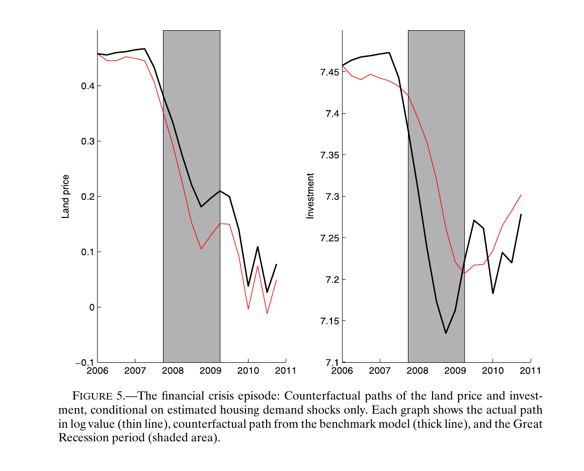
Two panels comparing actual and model-simulated paths of the log land price and log investment from 2006 to 2011; the counterfactual driven only by housing demand shocks tracks both collapses through the shaded 2008-09 recession — Figure 5, paper p. 1166: the financial-crisis episode. Actual paths (thin) vs. counterfactual paths from the estimated model fed only the housing demand shocks (thick); the observed declines — 25% in the land price, 22% in investment over 2007:Q3–2009:Q2 — are tracked “fairly well”, with the counterfactual generating declines of similar magnitude.

It tracks both collapses fairly well, with an investment decline of similar magnitude — not a match to the decimal, and the authors are unusually frank that this is one plausible mechanism among several, naming Gorton–Metrick’s repo run and Adrian–Shin’s intermediary balance sheets as things their model does not contain.

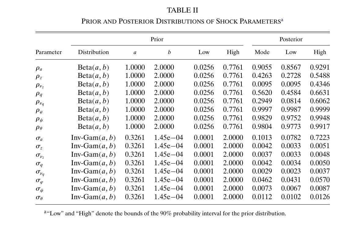
What a reader should push back on. Mostly one thing: the housing demand shock is the only object in the model that can move the MRS directly, so it was always going to absorb whatever land-price variance the other seven could not generate — and it absorbs about 90% of it. “Land prices are volatile because the taste for land is volatile” is uncomfortably close to a restatement of the data, and the estimate has the shape of a residual doing a job: persistence 0.9997 with a 90% interval of [0.9987, 0.9999], far outside the prior’s [0.026, 0.776], and a standard deviation of 0.0462, roughly ten times the technology shocks. The paper’s explanation is one sentence long: the land price is a very persistent series.

Table of prior and posterior distributions for the eight shock persistences and standard deviations; the housing demand shock row shows persistence 0.9997 and standard deviation 0.0462 — Table II, paper p. 1158: shock-process estimates. The housing demand shock is a near-unit root (posterior mode 0.9997) with a standard deviation an order of magnitude above the technology shocks — the number the strongest objection turns on.

The defences are real but partial. The authors are explicit that their contribution is the propagation mechanism, for which they need only some shock that lifts the land price on impact; an appendix offers a micro-foundation in which aggregating households who face idiosyncratic liquidity shocks and their own collateral constraints produces exactly such a term in the housing Euler equation, decreasing in micro loan-to-value tightness — so $\varphi_t$ can be read as household-side financial liberalisation rather than fickleness about lawns. It remains a labelled wedge. Three further soft spots, each conceded: the constraint is assumed always binding in a log-linearised model, which is awkward for the mid-2000s when it was presumably slackest, though the smoothed multiplier stays comfortably positive and a supplement adds nonlinear responses with an occasionally binding constraint; the loan-to-value ratio of 0.75 rests on imputing land as half of corporate real estate in data the authors themselves call extremely fragmentary and noisy, while the model’s implications for who holds the land cannot be confronted with data at all; and borrowed money becomes investment rather than entrepreneurial consumption only because the entrepreneur smooths his dividends — concave utility supplies that incentive and the estimated habit of 0.66 reinforces it, a requirement the paper flags and parallels to Jermann and Quadrini’s dividend adjustment costs, but a requirement nonetheless.

The runner-up surprise is a parameter. Investment adjustment cost comes out at 0.18, against 2.48 in Christiano–Eichenbaum–Evans, 5.48 in Smets–Wouters and about 26 in the Christiano–Motto–Rostagno model fitted to stock prices. A partial-equilibrium version of the mechanism shows why that is no accident: what drives investment is land value relative to the capital price, so the land price must outrun the capital price, which near-zero adjustment costs guarantee. The financial-accelerator literature needs capital to be expensive to install so that its price can swing; this model needs the opposite, and swings land instead.

Which leaves the tidy version of the finding: across 1975 to 2010 the American business cycle was substantially a story about firms whose ability to buy machines depended on what somebody else was willing to pay for a house. Not because houses are productive — the land under the plant contributes about two percent of output — but because they are seizable. The economy’s marginal investment decision was being made, roughly, by the appraiser.