Innovation, Growth, and Asset Prices

Howard Kung and Lukas Schmid, Journal of Finance 70(3), June 2015, pp. 1001–1037. Published version; no recorded talk, transcript or discussant, so this note works from the paper alone.

Howard Kung and Lukas Schmid’s paper is an answer to the question every long-run risk seminar eventually gets: where does $x_t$ come from? Bansal and Yaron (2004) get a large equity premium and a low risk-free rate out of a small, very persistent drift in expected consumption growth, priced by an Epstein–Zin (1989) investor who prefers early resolution of uncertainty. The drift is assumed. It is also nearly invisible in consumption data, which makes it a slightly uncomfortable thing to hang the equity premium on. Croce (2014) and others moved the drift into productivity, which helps production-based models, but it is still a latent process written down by the modeller.

Kung and Schmid’s move is to make the drift an equilibrium object. Put a Romer (1990) expanding-variety growth model inside an otherwise ordinary real business cycle model, let firms choose R&D, and the persistent component of productivity growth is just what the R&D sector decides to do. A transitory shock moves R&D, R&D moves the stock of ideas, and the stock of ideas is productivity. So a shock that dies out in the level of technology leaves a long, slow wake in its growth rate. The authors’ summary is four words long: “equilibrium growth is risky.”

The model: a free-entry condition that writes the long-run risk process

There are three kinds of firm. A competitive final-good firm combines physical capital, a fixed unit of labour and a bundle of $N_t$ differentiated “patents”, with a stationary ar(1) shock $\Omega_t$ on the labour-augmenting part. That shock is the only source of uncertainty in the economy, and there is no exogenous trend. Each patent is owned by a monopolist who turns one unit of final good into one unit of its input and sells it at markup $1/\nu$, so a patent is a dividend-paying asset: its value $V_t$ is current profit plus the discounted value of the patent next quarter if it hasn’t become obsolete, priced with the household’s stochastic discount factor. And a competitive fringe of innovators spends final goods on R&D to create new patents.

The innovation block is where the paper lives:

These are eqs. (8), (9) and (20): $N_t$ is the stock of patents (intangible capital), $S_t$ R&D spending, $\vartheta_t$ the number of new patents per unit of R&D, which innovators take as given, $\phi$ the obsolescence rate, $\chi$ a scale parameter, $\eta$ the elasticity of new patents to R&D, and $M_{t+1}V_{t+1}$ the discounted value of a new patent.

Read the last condition as a price. The cost of producing one patent is $1/\vartheta_t$ units of final good, and free entry sets that equal to what a patent is worth. This is Q-theory for ideas. The productivity $\vartheta_t$ rises with the existing stock $N_t$ (Romer’s knowledge spillover, which is what keeps growth from petering out) and falls with $S_t$ (congestion: when everyone does R&D at once, they duplicate each other). The authors note in a footnote that congestion acts like an adjustment cost on R&D, and without it the condition collapses to marginal Q equal to one, with R&D jumping around as violently as investment does in a frictionless model.

Then a parameter restriction does the quiet heavy lifting. The patent share $\xi$, the markup and the capital share have to satisfy $\alpha+\frac{\xi/\nu-\xi}{1-\xi}=1$, or the economy has decreasing or increasing returns and growth goes to zero or diverges (fn. 7). Impose it and the final-good technology aggregates to a textbook $Y_t=Z_tK_t^\alpha L_t^{1-\alpha}$, where measured tfp is $Z_t=\bar A(\Omega_tN_t)^{1-\alpha}$ (eq. 26). The Solow residual is the shock times the stock of ideas. With $\xi=0.5$ and $\alpha=0.35$, the restriction pins $\nu=0.6$, which is a markup of about 65%. That is the price of having a stationary growth model in which growth is chosen rather than assumed.

Now iterate the patent-value equation forward and the growth rate of $N$ becomes a function of discounted future patent profits (eq. 28). The authors read off two channels. The profit channel: patent profits are proportional to the final firm’s demand for patented inputs, which moves with $\Omega_t$, so profits are procyclical and as persistent as the shock. The discount-factor channel: with recursive preferences, more predictable consumption growth makes the pricing kernel more volatile, which makes patent values and therefore growth more volatile, which makes consumption growth more predictable. The paper calls that feedback “a long-run growth amplification mechanism”.

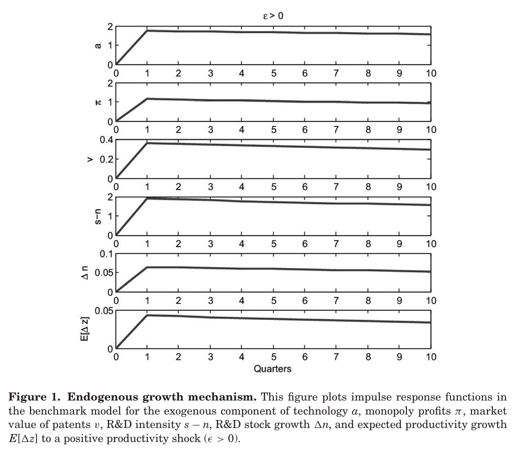
Figure 1 is the profit channel as a picture. A good shock raises demand for patented inputs, profits rise “persistently”, patent values rise, R&D intensity rises, the patent stock grows faster, and expected productivity growth goes up and stays up across the ten quarters plotted. The shock’s level effect is permanent (ideas, once created, keep raising productivity until they become obsolete) and its growth effect decays slowly. The model doesn’t need every shock to shift the growth rate forever; it needs shocks to shift it for a long time, and the free-entry condition provides that.

The punchline of Section II is an approximation. If the shock is persistent enough that its own growth rate is close to i.i.d., then

This is eq. (29): $Z_t$ is measured tfp, $\alpha$ the capital share, $\chi$ and $\eta$ the innovation parameters from above, and $S_t/N_t$ R&D spending over the R&D stock, which the authors call R&D intensity.

So expected productivity growth is, to a first approximation, a monotone function of a ratio you can download. It is worth being careful about what this does and doesn’t say. It is a statement about expected productivity growth, a different series from the Bansal–Yaron expected consumption growth, which inherits the persistence through general equilibrium but has its own volatility. And R&D intensity here is R&D over the R&D stock, not R&D over gdp.

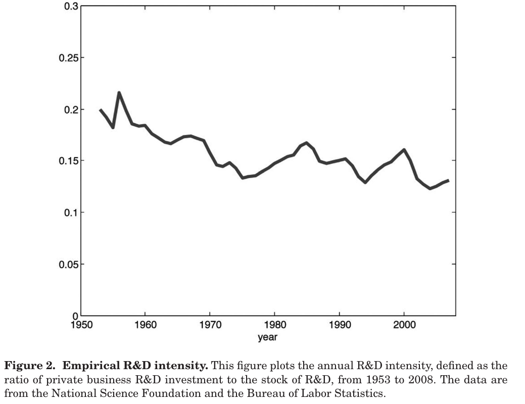
Figure 2 is that ratio in us data: nsf private business R&D over the bls R&D stock, 1953 to 2008. Its autocorrelation is 0.93, which is exactly the kind of number a long-run risk modeller wants to see. It also drifts down from about 0.20 to about 0.13 over the sample, which is a kind of number we will come back to.

The evidence: same shock, same consumption volatility, different economy

The calibration is quarterly, solved by second-order perturbation, with $\psi=1.85$, $\gamma=10$, an annualised shock persistence of $\rho^4=0.95$ and patent obsolescence of 15% a year (the bls R&D depreciation rate). The unusual choice is the targets. Instead of business-cycle moments, the authors target “growth cycles”: volatilities at periods of 100 to 200 quarters, 25 to 50 years, isolated with a band-pass filter, plus mean growth and the persistence of R&D intensity.

The comparison model is the cleanest thing in the paper. Hold R&D intensity constant and the same economy becomes a standard rbc model with an exogenous 1.90% trend. The authors then lower its shock volatility from 1.75% to 0.97% so that both models deliver the same 1.42% volatility of consumption growth. So the horse race is run at matched short-run consumption risk, not at matched shock variance, and whatever differs between the two columns is propagation.

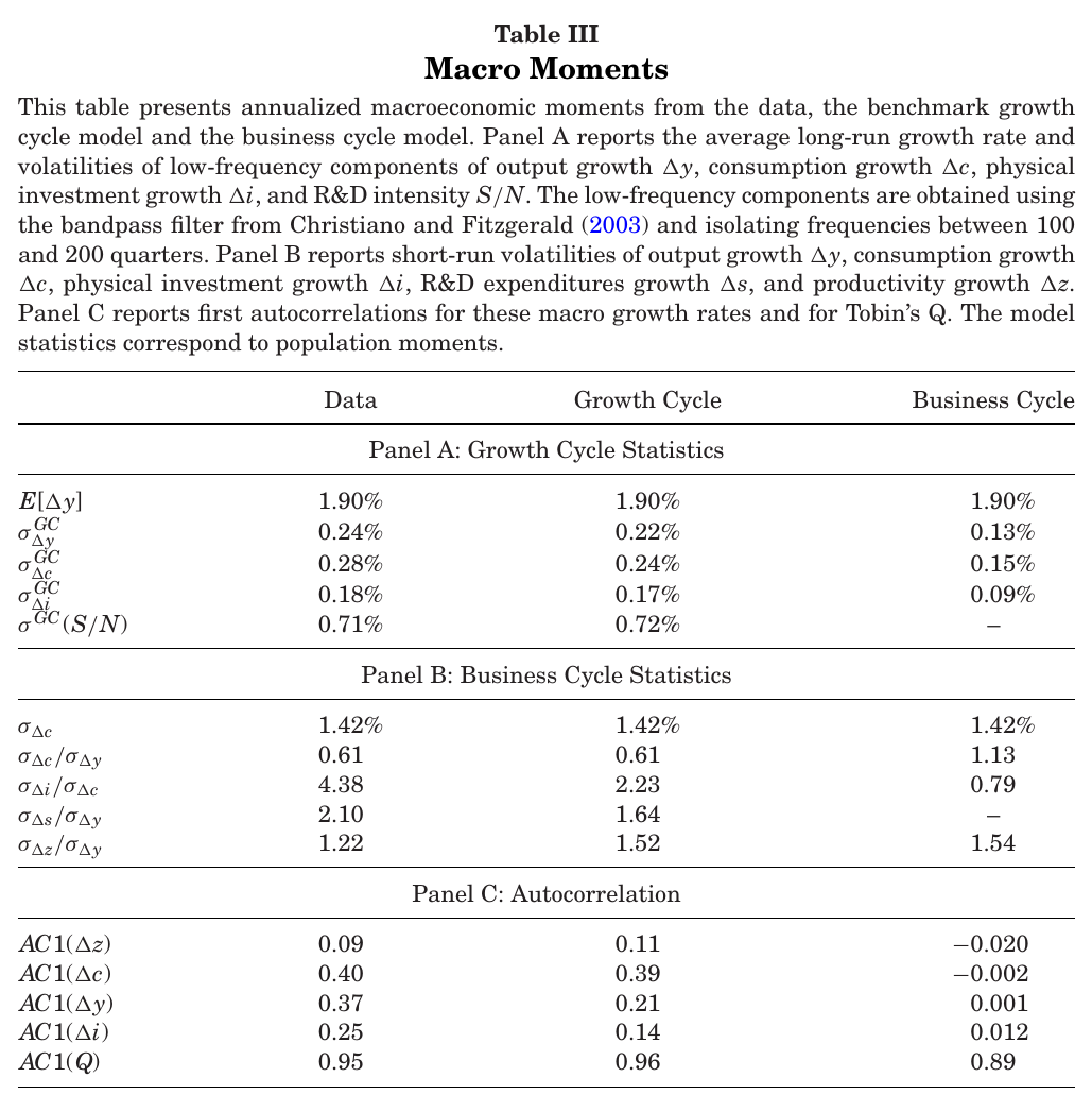
Table III shows what propagation buys. The first autocorrelation of consumption growth is 0.40 in the data, 0.39 in the R&D model, and −0.002 in the rbc twin. Output is 0.37, 0.21 and 0.001. The paper is entitled to the line it uses: the lack of persistence in growth rates “has long been identified as a weakness of the real business cycle model”, citing Cogley and Nason (1995), and here the same exogenous driver produces it in one column and not the other. Investment is too smooth in both models (relative volatility to consumption of 2.23 against 4.38 in the data), which the authors attribute to other shocks driving business-cycle investment.

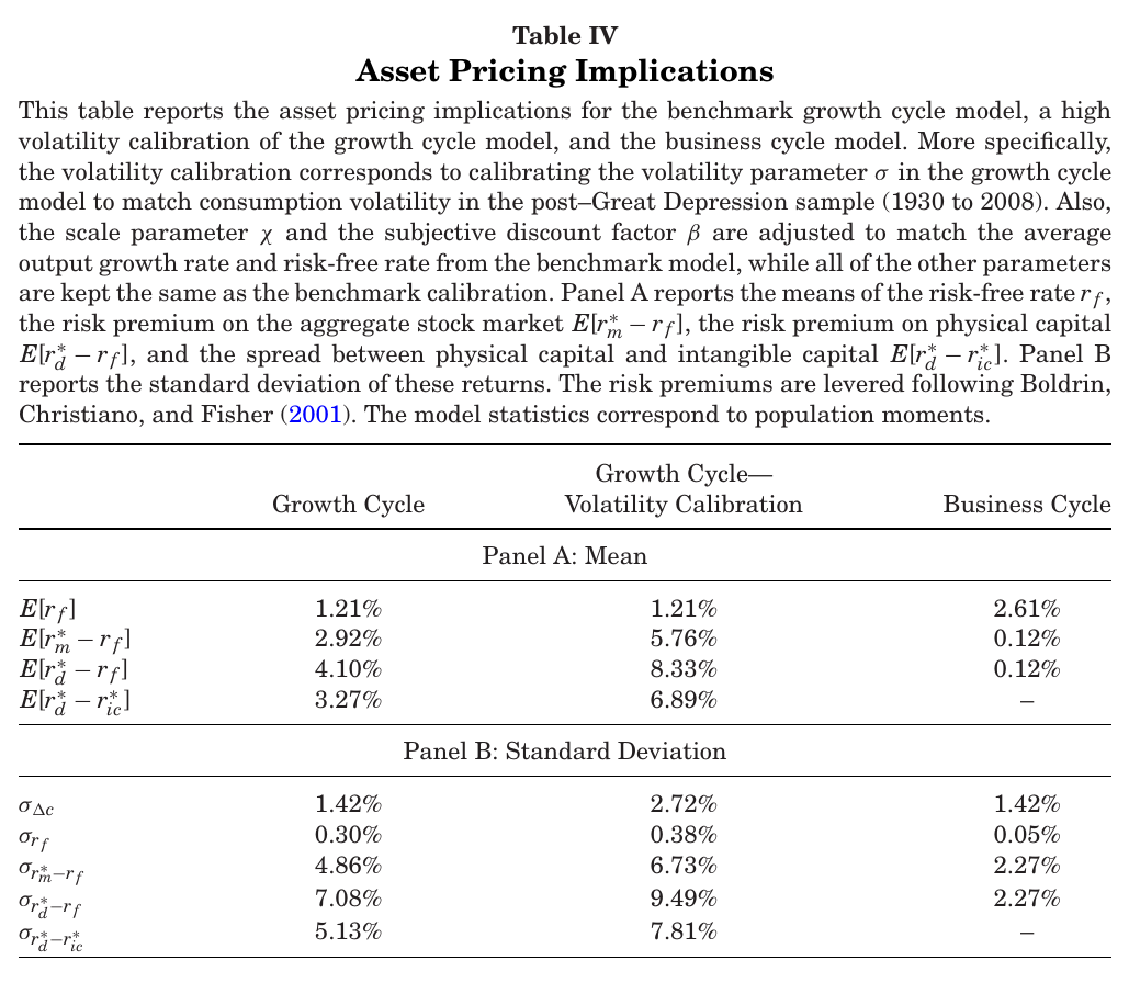
Table IV is the asset-pricing payoff. At identical consumption volatility, the levered equity premium is 2.92% with endogenous growth and 0.12% without it. The risk-free rate is 1.21% against 2.61%, because a household that knows slumps can last saves against them. The return on physical capital exceeds the market’s, and the spread between physical and intangible capital is 3.27%, which the authors “suggestively” relate to the value premium: physical capital is more exposed to the predictable component of growth than the patents whose creation drives it. They are candid that the mapping is loose, since growth firms in the data also own machines and in the model they own only patents.

The authors are also candid that the premia “do not rationalize their empirical counterparts entirely.” Their reading is that the model prices only the long-run productivity part of risk, and they cite Ai, Croce and Li (2013) for an empirical productivity-driven share of return volatility of about 6%, which they call “roughly consistent”. The third column gets a premium of 5.76%, but notice what it does: it matches consumption volatility in a sample that starts in 1930, so consumption volatility nearly doubles to 2.72%, and it retunes $\chi$ and $\beta$ as well to hold growth and the risk-free rate. It is a different economy, not a robustness check on the first.

The one surprising thing

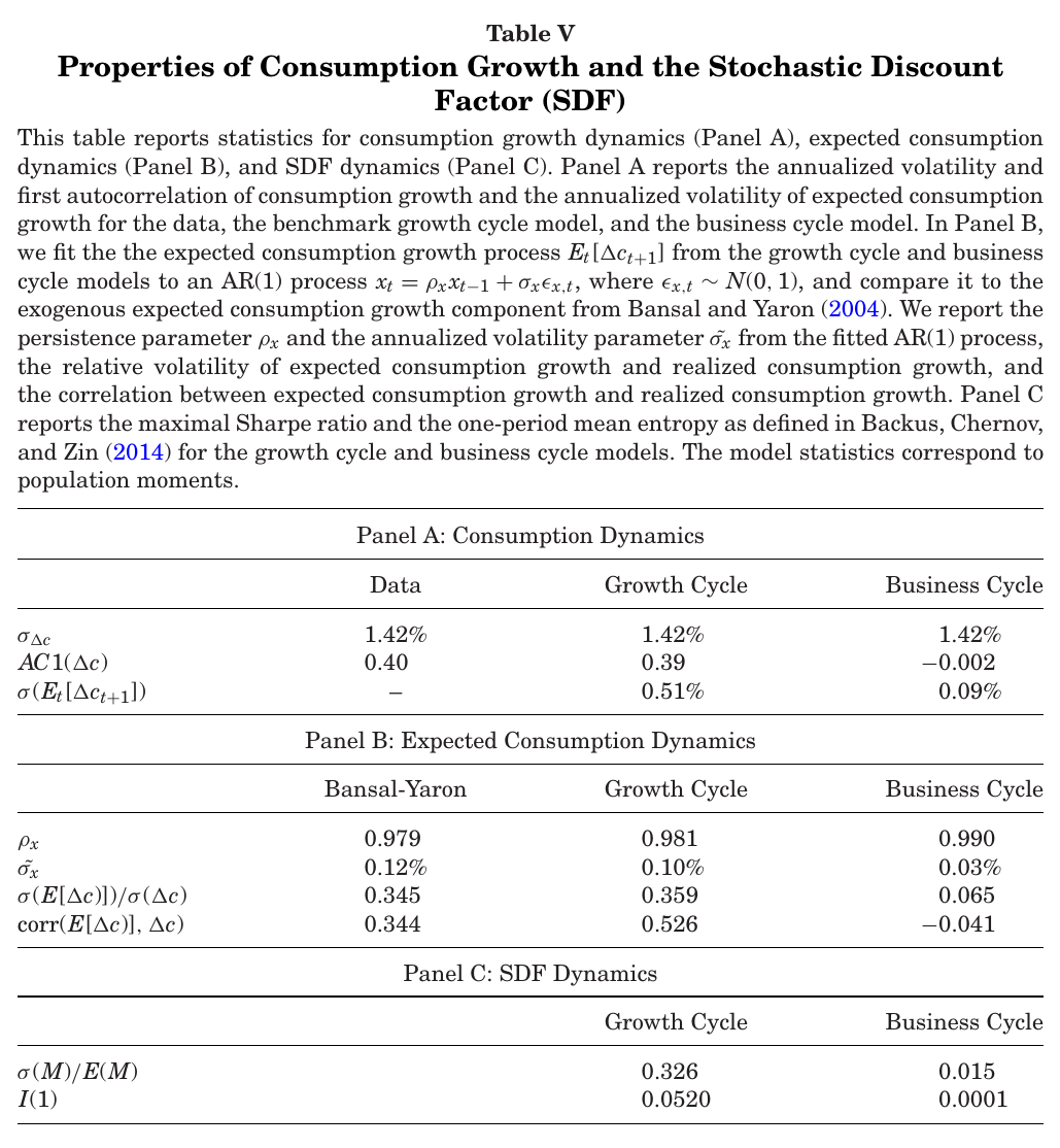
Now fit an ar(1) to the model’s expected consumption growth, the way you would if you were Bansal and Yaron writing down $x_t$. Table V reports persistence 0.981 and innovation volatility 0.10% for the R&D model, against 0.979 and 0.12% for Bansal and Yaron’s parameterisation. Nobody targeted those numbers. The model was tuned to a handful of 25-to-50-year volatilities and the persistence of R&D intensity, and the latent process that the long-run risk literature had simply assumed drops out of an R&D free-entry condition looking much like the assumed one. The authors’ own phrasing is the right one, “close to” and “slightly more persistent but slightly less volatile”, and the table doesn’t say at what frequency the persistence is measured, so “close” is as far as it should be pushed. Still, it is close.

The rest of Table V is the same contrast seen from the pricing kernel. The volatility of expected consumption growth is 0.51% against 0.09%; the maximal Sharpe ratio, $\sigma(M)/E(M)$, is 0.326 against 0.015. The second number is far below even the power-utility benchmark, and the paper explains why: in the rbc model consumption growth is slightly negatively autocorrelated, so short-run and long-run news hedge each other. In the R&D model a bad shock lowers consumption today and expected growth tomorrow (their correlation is 0.526), so the two pieces of bad news arrive together, and a household with a preference for early resolution hates that. Same consumption risk, one model prices it at 0.12% and the other at 2.92%. That is the whole long-run risk argument in a controlled experiment.

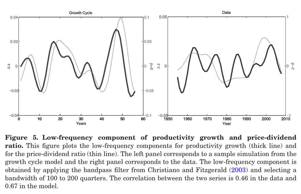
Valuations follow. Band-passed to the same 25-to-50-year window, productivity growth and the price-dividend ratio move together, with correlation 0.67 in the model and 0.46 in the data (Figure 5). In the model, though, that comovement runs through expected cash flows: “the benchmark model generates little time-variation in risk premia.” The authors mention an extension with stochastic volatility in the shock that “replicates the predictability evidence well”; it is not reported.

The forecasting regressions

If R&D intensity is the observable face of long-run risk, it should forecast growth. Section III.E runs that test on annual data from 1953 to 2008: cumulative growth over one to five years on log R&D intensity (or R&D stock growth), with Newey–West errors.

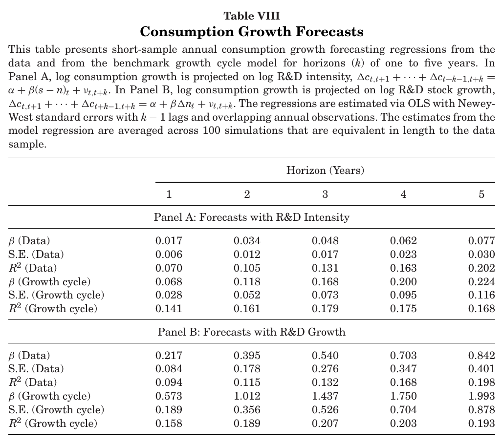
In Table VIII the data slope of consumption growth on R&D intensity rises from 0.017 at one year to 0.077 at five, each about two and a half to three standard errors from zero, and the $R^2$ climbs from 0.07 to 0.20. Model simulations of sample length give $R^2$ in the same neighbourhood, 0.14 to 0.18. The same exercise for output and productivity (Table IX) runs in the same direction. The authors’ verdict, “qualitatively, the model replicates these patterns well”, is chosen with some care, and the qualifier is earning its place: in Table VIII the model’s consumption slopes on R&D intensity are about three to four times the data’s.

This is the part of the paper Franceschini (2026) picks up. He keeps the claim that R&D drives a persistent component of productivity but argues that the ratio used here behaves like a near-unit-root process in longer data, and replaces it with a cointegrating residual of R&D on tfp and employment.

Objections and limits (the reader’s own; there is no discussant)

The forecasting regressor is a trap of the familiar kind. R&D intensity has autocorrelation 0.93 and trends down across the sample, the regressions use 56 annual observations with overlapping horizons up to five years, and consumption and productivity growth also slowed over the same decades. Stambaugh-style small-sample bias and a shared trend could carry much of that $R^2$, and there is no out-of-sample test and no horse race against other slow-moving predictors. Matching the model’s small-sample $R^2$ shows the model could produce such regressions, not that the data’s come from the model’s channel.

Prediction is also not causation, and the model itself says so. In the model R&D responds to expected patent profits; in the world any forward-looking investment anticipates growth. Nothing in the evidence distinguishes “R&D causes future growth” from “R&D sees future growth coming”, and the paper doesn’t try.

The growth-cycle calibration targets 25-to-50-year volatilities in a 56-year sample, which is at most two cycles of the longest period. Several parameters are tuned directly to those moments ($\eta$, the adjustment cost, the shock volatility), the shock persistence is chosen to match the persistence of R&D intensity, and no sampling uncertainty is reported for the targets. The authors’ best answer is the comparison model: the same $\rho$ gives near-zero growth persistence without endogenous R&D, so what they are claiming is the transmission, not the shock. That answer is a good one.

The premium is modest, appears only after leverage, and the table has no data column to compare it with. The model’s price-dividend ratio moves for cash-flow reasons in a literature that mostly finds it forecasts returns. Dividends are macro net corporate dividends, their volatility in the model is about half the data’s, and labour is fixed. The value-premium reading treats “growth firms” as pure patent portfolios.

Finally, a few slips a replicator will hit. Table II’s rows labelled $\nu$, $\phi$ and $\zeta$ run over values (1.63–1.67, about 0.96, and 0.05–0.09) that don’t match Table I’s parameters, and read most naturally as the markup, the survival rate and something unexplained. The text says higher $\eta$ raises growth while Table II has it falling. Eq. (27) as printed puts $\chi$ inside the expectation with the wrong exponent; eq. (28) is consistent with the derivation. None of these touch the results.

All of which leaves the paper’s real contribution exactly where the authors put it. The authors don’t claim it fits the equity premium better than an exogenous long-run risk model; the pricing mechanism, they say, is Bansal and Yaron’s. It takes the one ingredient that long-run risk models assume and nobody can see, and shows that an ordinary growth model with monopoly profits and free entry produces something very like it unprompted, along with a ratio you can look up. That the ratio then turns out to have trouble staying stationary is, in a way, the most long-run-risk thing about it.

References