The Demographic Cliff and the Market for Higher Education: Implications for Public Finance

Dirk Krueger, Alexander Ludwig and Irina Popova have a model in which America’s post-2008 fertility decline leaves the country, per head, somewhat richer and cheaper to govern, and the reason is the structure of the college market. Not higher education in general. The structure: a ladder of colleges at every quality level, each pricing students by ability. Take the ladder away, leave everything else alone, and the good news turns bad.

Before the mechanism, a warning about which paper this is, because there are two of them. The public document is the 30 April 2026 draft. It compares steady states: population growth goes from 1% to 0% and the total population ends 30.6% smaller (p. 45, Table 4 notes; page numbers here are pdf pages). The draft says outright that transitions are deferred “to future versions of this paper” (p. 48), and a footnote says it abstracts from intergenerational transfers (fn. 1, p. 6). Irina Popova presented a newer version on 18 September 2026 at the nber virtual workshop on the macroeconomic effects of population aging, from slides dated September 2026. That version runs a full transition from 1950 to 2200, with households learning about the cliff in 2010 and 2086 as the year of interest. It links young people’s starting wealth to bequests, and it adds a representative-college counterfactual. None of the talk’s headline numbers are in the April draft, and on output per head the two versions disagree in sign: −0.63% in the paper’s steady state (Table 5, p. 47), +2.30% in the talk’s 2086 (01:13:27). Every number below is labelled paper or talk.

Here is the part the two versions share, and it is the good part. A selective college is a firm that buys one of its main inputs from its own customers. The product is quality, and quality is made from two things: money spent per student and the ability of the students sitting next to you. So a high-ability applicant is a customer and also a supplier, and the college pays her for what she supplies by charging her less. This is the Cai and Heathcote (2022) “club” model of the college market, and it is not a metaphor laid over the paper. It is the paper’s price system. Once you see a merit discount as a factor payment, the cliff’s effect on college follows almost mechanically.

The short version goes like this. You run a middle-quality college. Aging makes skilled labor scarcer and better paid, so more 18-year-olds decide college is worth it, and the ones who change their minds are the marginal ones, who are on average weaker than the students you already had. To hold your quality fixed with a weaker class, you need to spend more per student (tuition goes up for everyone), and your strong students are now scarcer, so you pay them more (their discount goes up). The weak pay more, the strong pay less, and some of the strong move up the ladder to a better college that now wants them more.

The model

The economy is an overlapping-generations life-cycle model in four-year periods, with entry at 18. The model’s colleges are cells indexed by a continuous quality $q$ and a major $p$, non-Stem or Stem. Quality zero means no college. Each cell has free entry, constant returns and zero profits, plus a fixed cost $\kappa(p)$ per student that is higher for Stem. A college chooses spending per student $i$ and the share $\eta$ of high-ability students it admits, and the first-order condition defines the price that does all the work:

Those are eqs. 22 and 24 in the paper. $\bar e$ is the mean ability of the students in the cell, $A_q$ is quality tfp, $\theta$ is how much quality depends on classmates (0.5 in Table 1, p. 28), $v(q,p,e)$ is revenue per student of ability $e$ (tuition plus subsidy), and $d$ is the discount per unit of ability that clears each cell. The authors are explicit that the discount is the whole equilibrium: “All other equilibrium elements as well as the qualitative features of the equilibrium then follow from the properties of d(q, p)” (p. 15). In the talk Popova put it as “base tuition and an ability discount” being “the prices that clear the college market” (00:59:20).

Substitute the zero-profit condition back in and you get tuition by type:

These are eqs. 49–50 (p. 24): $s$ is the public subsidy and $\Delta e = e^h - e^l$. Read them as a cost-sharing rule. Everyone pays the fixed cost and the spending, net of subsidy. Then the low-ability student pays a surcharge proportional to how many high-ability classmates she is getting, and the high-ability student gets a rebate proportional to how many low-ability classmates she is carrying. When $\eta$ falls, $i$ and $d$ both rise. Low-ability tuition rises unambiguously, and high-ability tuition could go either way. The gap between the two responses has a fixed sign (eq. 53), so the schedule always rotates against the weaker student. Tuition is linear in ability and does not depend on family resources.

On the other side of the market, households differ in ability (two levels, 1.0 and 0.375), in residence (in-state students get the subsidy, 49% of tuition) and in initial resources $b$. They pick a cell or no college, face dropout risk that falls with quality, and can borrow at most 45,000 dollars per four-year college period (Table 1, p. 28). After college they live a standard consumption–savings life. Production has three labor inputs: non-college, non-Stem college and Stem college. Each is nested with capital with its own substitution parameter, and $\rho = 0.33, -0.11, -0.43$ respectively (eq. 38, p. 17; Table 1). That ordering is the model’s capital–skill complementarity: Stem labor is the most complementary to capital, so capital deepening favors it. The government adjusts the labor-tax level every period to balance its budget. Pensions are pay-as-you-go and balance through the replacement rate. In the talk’s version, non-education spending scales one for one with population (01:03:20), which is a quiet but important assumption: a smaller country is assumed to need proportionally fewer roads and soldiers.

Unlike Cai and Heathcote, the paper treats college as an investment good under credit frictions that bind without being severe, a case the authors say nobody has solved numerically before (p. 25). What matters for the results is that the borrowing limit binds for some marginal students. It comes back when the ladder is removed.

The cliff, twice

Anyway, here is what happens when you push fertility off the cliff, first in the April draft. Its steady-state experiment is a 1% to 0% drop in population growth with a 30.6% smaller population. The long-run capital–labor ratio rises, the interest rate falls 0.86 percentage points, and wages rise 4.62% for non-college workers, 4.92% for non-Stem graduates and 5.02% for Stem graduates (Table 4, p. 45). The falling pension replacement rate adds its own push, since a worse pension makes your own human capital a better retirement plan (p. 40). Non-attendance falls by “more than six percentage points,” and the new students go mostly to middle-quality colleges (p. 40). The tuition schedule rotates the way the equations say it must: at middle quality, low-ability tuition rises “up to about 2.5% for non-Stem majors and around 2% for Stem,” and high-ability tuition falls “more than 2%” (p. 42). The labor tax falls 0.53 points. Output falls 31.00%, which is mostly the 30.6% of people who are no longer there, and output per head falls 0.63% (Table 5, p. 47).

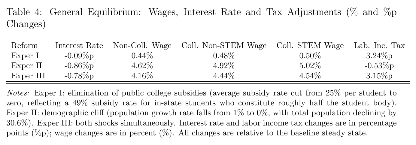
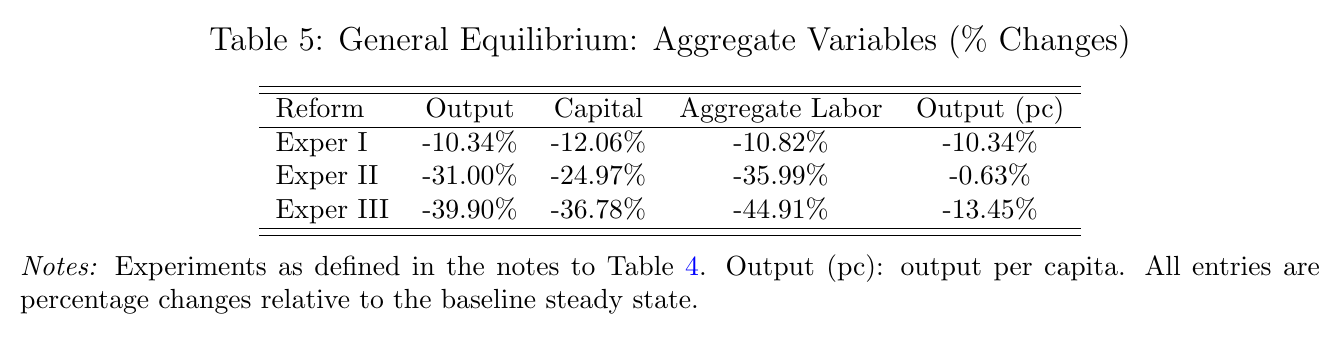
The story is advertised as capital–skill complementarity, but the wage row is modest about it: the Stem–non-college wedge is 0.4 points on top of a large common increase, and the paper concedes the response “remains relatively similar” across groups (p. 46). The ρ ordering sharpens the enrollment response. The level of wages, the lower interest rate and the thinner pension do most of the work.

The paper also has an experiment the talk skipped, and it is the paper’s actual policy point. Removing public college subsidies raises the labor tax 3.24 points on its own. Removing them during the cliff raises it 3.15 points, which is more than the 3.24 − 0.53 = 2.71 you would get by adding the two separately (Table 4; p. 46). The cliff’s fiscal cushion is enrollment, and subsidies pay for enrollment, so cutting subsidies removes the cushion exactly when it is needed. The authors call the buffer “fragile” and “enrollment-driven” (p. 5), and given which federal funding cuts they have in mind, it is the sentence in the draft most likely to be quoted.

Then the talk, which is a different set of numbers from a different exercise. In the transition, the adult population is about 21% smaller than the no-cliff baseline in 2086, and the working-age population ratio is about 67% against 72% (01:08:35–01:09:15). (Earlier, at 00:52:31, she said “from about 78%”; the slide says 72%.) The gap peaks in the 2080s, which is why 2086 is the year of interest. Middle-quality tuition rises about 2.2% for low-ability students and falls about 1.5% for high-ability ones (slide 12; “about 2%” in speech, 01:11:30). The interest rate is a quarter point lower, and wages are up 0.9% for non-college, 1.4% for non-Stem and 1.5% for Stem graduates. Enrollment is 8.69 points higher, the labor tax is 1.15 points lower and output per head is 2.30% higher.

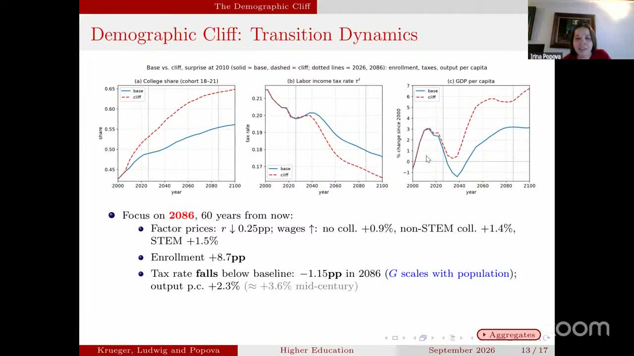
“Mildly positive in per capita terms and more than self financing” (01:13:40) is the talk’s headline. Notice that the fiscal direction is the same in both versions, since the tax falls in the steady state too. What changed is whether output per head rises. That depends on a channel the April draft does not have, which I come to below.

One more place where the versions disagree is the major mix. In the paper’s steady state, the Stem share falls at middle-quality colleges and in aggregate, because the lower-ability entrants avoid the harder major: “the overall proportion of students choosing Stem falls despite the increase in total college attendance” (p. 42; Figure 7d, p. 41). In the talk, the mass shifts toward middle and high quality “and slightly more so to Stem” (01:10:12), and the conclusion lists “a slight shift towards Stem education” (01:18:52). The talk’s claim is read off stacked enrollment bars, with no Stem-share panel shown. Both can be true, since the transition has a bequest channel and a time path the steady state lacks, but anyone arguing that the baby bust helps the Stem pipeline should say which version they are citing.

Take away the ladder

This is the talk’s main addition and the most interesting exhibit. Replace the whole distribution of colleges with one representative college at the mean quality $\bar q$, offering one blended major and pricing by the same rule, and run the same cliff (01:14:06).

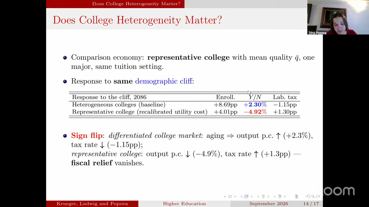
Enrollment still rises, by 4.01 points instead of 8.69, but output per head now falls 4.92% and the labor tax rises 1.30 points. Here is some rough arithmetic of my own, not the authors’. The age structure alone costs about 7% of output per head, since 0.67/0.72 ≈ 0.93. The gap between the two college markets is 2.30 − (−4.92) ≈ 7.2 points. So in this model the shape of the college market is worth about as much as the entire age-structure effect of the cliff.

Popova’s explanation has two parts (01:15:08–01:15:42). With one college, the intensive margin is absent by construction: students already enrolled cannot move up a quality ladder or switch into Stem, because neither exists. More surprisingly, the extensive margin is weaker too. “With only one representative college entry cost is relatively high for borrowing constrained marginal students,” because the only thing for sale is the mean-quality bundle, at the mean-quality price. In the heterogeneous economy, a marginal student with a binding borrowing limit can buy a cheap, low-quality seat. In the representative economy she has to buy an average seat, can’t finance it, and stays out. The ladder is valuable partly because it has cheap rungs at the bottom.

The skeptical note is that the representative college comes with a “recalibrated utility cost,” which the slide does not specify. So this compares two calibrated economies, not one economy with a margin switched off. A direct utility cost is exactly the kind of parameter that can move an extensive margin by four points, and the talk did not say what the recalibration did to it.

Grandparents are part of the mechanism

The talk’s other addition is on the resource side. In the September version, the mean of young households’ initial resources “is a function of end of life bequests” (00:59:59). An aging population leaves estates to fewer heirs, so under the benchmark scheme inheritances per head are about 9% higher by 2086 (01:16:09). The scheme is calibrated to transfers received by young households in the 2013 psid Rosters and Transfers supplement. More money in the hands of 18-year-olds relaxes exactly the borrowing constraint that the representative-college experiment showed to be binding. Slide 15 then varies how strong this channel is, in both college markets.

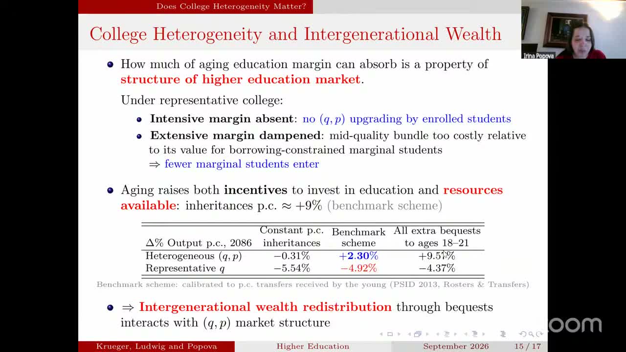
Hold inheritances per head at their baseline path, and the heterogeneous economy’s +2.30% becomes −0.31%: “slightly negative. So effectively it disappears” (01:17:17). Send all the extra bequests to 18- to 21-year-olds, and it becomes about +9.6%. In the representative-college economy the same range of schemes moves output per head only from −5.54% to −4.37%. Extra money helps a lot when there is a ladder to spend it on and not much when there isn’t. (Popova’s spoken reading of the table at 01:17:46 is garbled in the captions; the numbers here come from the slide.)

Put the two tables side by side, and the surprising thing about the talk is clear. The upbeat headline, that a 21% smaller adult population leaves Americans richer per head and paying lower taxes, needs both the college ladder and the bequest channel. Without the ladder, the sign flips. Without the bequests, the gain disappears. The April draft has the ladder but no bequest link (initial resources there are exogenous), and its steady-state −0.63% sits near the talk’s constant-inheritance cell (−0.31%). The exercises differ, so this is a resemblance, not a reconciliation, but it suggests that most of the sign difference between April and September is the grandparents. The bequest mechanics exist only on slides, so for now you can’t check how the windfall is divided among heirs, and the “all extra bequests to ages 18–21” column is best read as a bound rather than a forecast.

What the room asked

There was no discussant. Clarifying questions came during the talk, a short Q&A followed, and Dirk Krueger answered some questions in the Zoom chat, which the recording does not capture (01:19:59). Three exchanges survive.

During the benchmark slides, an unnamed participant asked whether the panels were data or model, and whether the model’s $q$ could be mapped to anything measurable (01:05:09). Popova said those panels are untargeted model output used as validation. On measuring quality, “there’s no like clear unambiguous way,” though the tuition gradient is “very close” to what ipeds data show (01:06:04). That is a fair answer and a real limitation: the object that carries the results has no agreed empirical counterpart.

In the Q&A, a participant the chair called “Adrian”, presumably the organiser Adrien Auclert, asked two things (01:20:23). Is there an indirect test, such as which colleges are shrinking or closing along the quality dimension and how tuition is responding? And how does immigration, including of students, interact with all this? On the first, Popova said contemporaneous validation is hard, but past fertility fluctuations or state-level college markets might work. On the second, immigration is “in our agenda”: Stem immigration, and foreign students as a tuition source (01:21:18–01:22:14). A co-author then added a point about what the model can say (01:22:39). The captions don’t name him, but given the chair’s thanks to Krueger a moment earlier, it was plausibly Krueger. Every quality tier loses students, he said, and the middle and top lose proportionally fewer. Under constant returns, though, the model can’t say whether that means fewer colleges or smaller ones: “we cannot make statements about you know Stanford shutting down or Penn shutting down” (01:23:36). That needs fixed costs. This is an honest limit worth stating plainly: the model that reads the cliff through the college market has no college closures in it. The closures the talk opened with, about 100 institutions, “mostly relatively low quality two-year institutions” (00:53:14), show up in it only as a shrinking segment.

Adrian’s follow-up was the best exchange of the session (01:24:13). The cliff hasn’t arrived, but the transition starts in 1950, so the model already makes predictions for every past year of demographic change, and those can be compared with how enrollment actually moved along the quality distribution. The co-author agreed: “that’s a fair point… We didn’t so far but we could” (01:25:10). Popova added that the constant-returns model is “inherently about the long run” (01:25:39). Both points hold. They also mean that a model which has been simulating American college markets since 1950 has not yet been checked against any of that history.

The flattering corollary

Popova ended with the cross-country implication: countries with different higher-education systems “may experience very different effects of population aging on the skill composition of their workforce” (01:19:33). That is true within the model, and it is also a flattering thing to say about the American system, whose sprawl is usually described as a problem. The claim, taken seriously, is that America’s fiscal defence against the baby bust has two parts. One is a college market with a seat at every price, including many cheap seats that nobody ranks. The other is a generation of parents whose estates are split among fewer children. Each of those appears in the model as a margin. Neither is usually counted as fiscal policy.

References