Population Aging and Economic Growth: From Demographic Dividend to Demographic Drag?

Rainer Kotschy and David Bloom’s paper on aging and growth turns out to be mostly about one number, and it isn’t an elasticity. It is the age at which you decide someone is old. A quick note on versions first. The public paper is the August 2023 nber Working Paper 31585, under the title above. At the nber workshop on the macroeconomic effects of population aging in September 2026, Kotschy presented it as “Population Dynamics and Economic Growth” and showed some material the 2023 draft doesn’t have. The main example is a regression slide with a no-controls column, which I’ll mark as talk-only when it comes up. The projections he showed look like the paper’s own figures, not new estimates.

Division is not a mechanism

Start with the part that is true by construction. Income per capita equals output per worker times the share of the population that works. If the working-age share goes up 10 percent and output per worker stays put, income per capita goes up 10 percent. Nobody saved more, nobody innovated, nobody moved to a city. You just divided by a smaller number of dependants. In the paper’s notation (eq. 3, p. 8):

Here $\tilde y$ is income per capita, $y$ is income per worker, $w = L/N$ is the working-age share, $A$ is tfp, and $k$ and $h$ are physical and human capital per worker.

Take logs and first differences and the coefficient on $\Delta \ln w$ in a growth regression is pinned at exactly one. The demographic-dividend literature has long estimated coefficients above one and credited the excess to behaviour. A bulge of prime-age workers saves, invests and innovates, so a rising working-age share does more than the arithmetic. Kotschy put it plainly in the talk (04:38:54): when the estimate exceeds the restriction, “people save more, people innovate more, um people might even trade more.”

The paper keeps that identity as a restriction and tests it. tfp follows a conditional-convergence process toward a potential built from world time effects, lagged human capital and covariates (institutions, life expectancy at birth). Lagged productivity is proxied by lagged income per worker, which the authors rewrite in per-capita terms. That adds a level term in the lagged working-age share whose coefficient is restricted to equal the convergence speed. The estimating equation (eq. 7, p. 9) is:

$\lambda$ is the convergence speed, $\tau_t$ the frontier time effects, $x_{it}$ the covariates, $\theta$ a Nelson–Phelps (1966) term that lets high-human-capital countries adopt technology faster, and $\varepsilon_{it}$ the productivity shock. The theory makes two predictions: a coefficient of one on $\Delta \ln w_{it}$ and a coefficient of $\lambda$ on $\ln w_{it-1}$. If the data reject them, either the specification is wrong or behaviour is doing work beyond the accounting.

Growth in the working-age share is obviously endogenous. People migrate toward booms, and booms change fertility. So the authors instrument it with the log population share aged 15 to 19 five years earlier. That is the cohort about to age into the working ages, fixed by births about two decades back. Kotschy stated the exclusion restriction in plain terms (04:37:56): “people do not systematically anticipate productivity shocks.” The data are a panel of 145 countries in five-year steps from 1950 to 2015. The appendix reports robustness checks with longer cohort lags, fertility, and an outflow instrument.

The talk-only slide, and the coefficient that goes back to one

The talk showed this more cleanly than the 2023 draft does. Slide 12 puts the demographic-dividend specification without controls next to the full model.

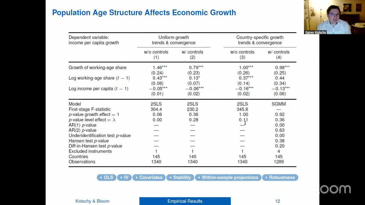
Without controls, 2SLS gives a growth effect of 1.46 (s.e. 0.24), and a coefficient of one is rejected at the 10 percent level (p = 0.06). The level effect is also above its restriction. Add capital and human capital and the growth coefficient falls to 0.79. Unity is no longer rejected. That is the paper’s Table 3.

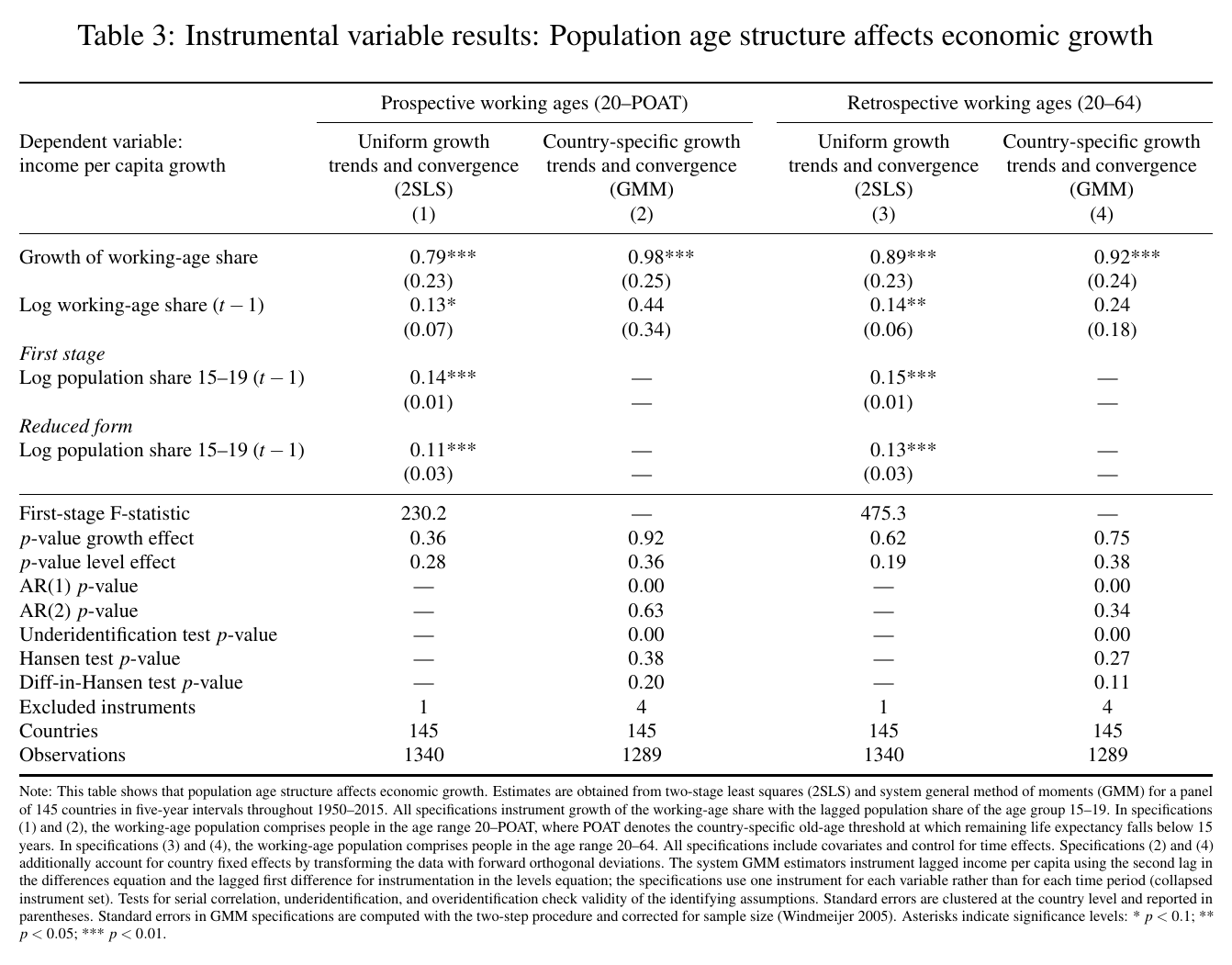
All four columns land near one. Prospective ages give 0.79 with 2SLS and 0.98 with system gmm. Retrospective ages give 0.89 and 0.92. The p-values for the test of unity are 0.36, 0.92, 0.62 and 0.75. The first stages are strong (F of 230.2 and 475.3), and the level effects are not distinguishable from $\lambda$ either. The paper’s ols estimates come in below one, which the authors read as endogeneity. The instrument moves them back up. As Kotschy summarised it (04:39:58), once capital and education are in, “what we have left is the accounting effect.”

This is a strange thing to present as a result. The regression’s big finding is that it cannot reject an identity. It is also a useful result, and the reason is worth stating carefully. The behavioural channels haven’t vanished. They run through capital accumulation and schooling, and the model now carries those as separate regressors. So the effect of age structure holding capital and education fixed is just division. That makes the projections very transparent, as long as you remember that capital and education are being projected along a separate path. The authors check the capital side in an extension. When the capital stock responds endogenously to age structure (eq. 8, p. 22), the drag gets larger and the health offset shrinks from about one-half to “roughly one-third” (p. 22).

Once the coefficient is one, the model doesn’t decide how much aging slows growth. The measured change in $w$ decides it. And $w$ depends entirely on where you put the upper edge of “working age.”

Where old age starts

The conventional cutoff is 65, fixed, which amounts to assuming that a 65-year-old in 2050 functions like a 65-year-old in 1970. The paper states the problem directly: in the United States, life expectancy at 65 “rose from 15 to 19 years in 1970–2020 and is projected to reach 23 years by 2050” (p. 5). If 65 was the right place to call someone old in 1970, keeping it there adds people to the measured old-age population who would not have counted as old by the 1970 standard.

The alternative comes from Ryder (1975) and from Sanderson and Scherbov (2017). They define the prospective old-age threshold, or poat, as the age at which remaining life expectancy falls below 15 years. The 15 is chosen so the threshold matched 65 in low-mortality countries around 1970. For the United States the poat was about 65 in 1970 and 72 before Covid, and it is projected to reach 76 by 2050 (p. 5). Working age then runs from 20 to the poat, not 20 to 64. The paper checks that the threshold measures more than mortality. Conditional on country and time fixed effects, it moves with life expectancy at 65, grip strength and word recall, and against health deficits per person aged 50 to 79 (Table 1, p. 6). The grip-strength and recall correlations rest on a small subsample of countries, but they point the same way as the rest.

A clarifying question early in the talk asked how big the move is (04:29:48). Kotschy answered “between 5 and 10 years older than 65,” so 75 in some countries and “67 or so” in others. Then he added the part that matters later: in non-oecd countries it “can even be slower than 65. So you could be at 60 or 55.” The threshold can go below 65 as well as above it. Measured prospectively, rich countries look younger and poor countries look older. Among oecd countries, the prospective and retrospective working-age shares are about 5 percentage points apart by 2050, which is about 10 percent in relative terms (p. 7; talk at 04:30:52).

Three scenarios that differ in one variable

The projection exercise is kept simple. The authors fit the model on 1950–2015 and project 2020–2050 under three scenarios. The only thing that varies across them is $w$. In the first, the working-age share is frozen at 2015 levels, so there is no aging. In the second it follows projections for ages 20–64. In the third it follows projections for ages 20 to poat. Trends, education projections and the capital path are the same in all three. So, as Kotschy said (04:42:32), the levels don’t mean much and the differences between scenarios are the result. Scenario two minus scenario one is the drag from cohort structure. Scenario three minus scenario two is how much of that drag improving health could offset.

For the oecd as a group, the no-aging scenario gives 2.5 percent annual growth in income per capita. The retrospective scenario cuts that by a third to about 1.7 percent. The prospective scenario cuts it by a sixth to 2.1 percent, given an average rise in the poat of 4.5 years over 2020–2050 (p. 19). So the drag is about 0.8 percentage points a year measured the usual way and about 0.4 measured the health-adjusted way. Health “can cushion perhaps one-half of this demographic drag” (p. 19). Note that these are simple averages of cumulative 30-year growth, not compounded rates (footnote 3, p. 19). For 2020–2030 alone, the retrospective drag of 0.54 points is close to the 0.6 that Maestas et al. (2023) get from variation across U.S. states. The prospective version gives 0.26 (p. 4). Looking at all 145 countries, aging slows growth in 70 of them. The paper calls that “virtually all those whose working-age shares contract” (p. 4; talk at 04:49:52).

The country breakdown is the key exhibit, and it shows what the average leaves out.

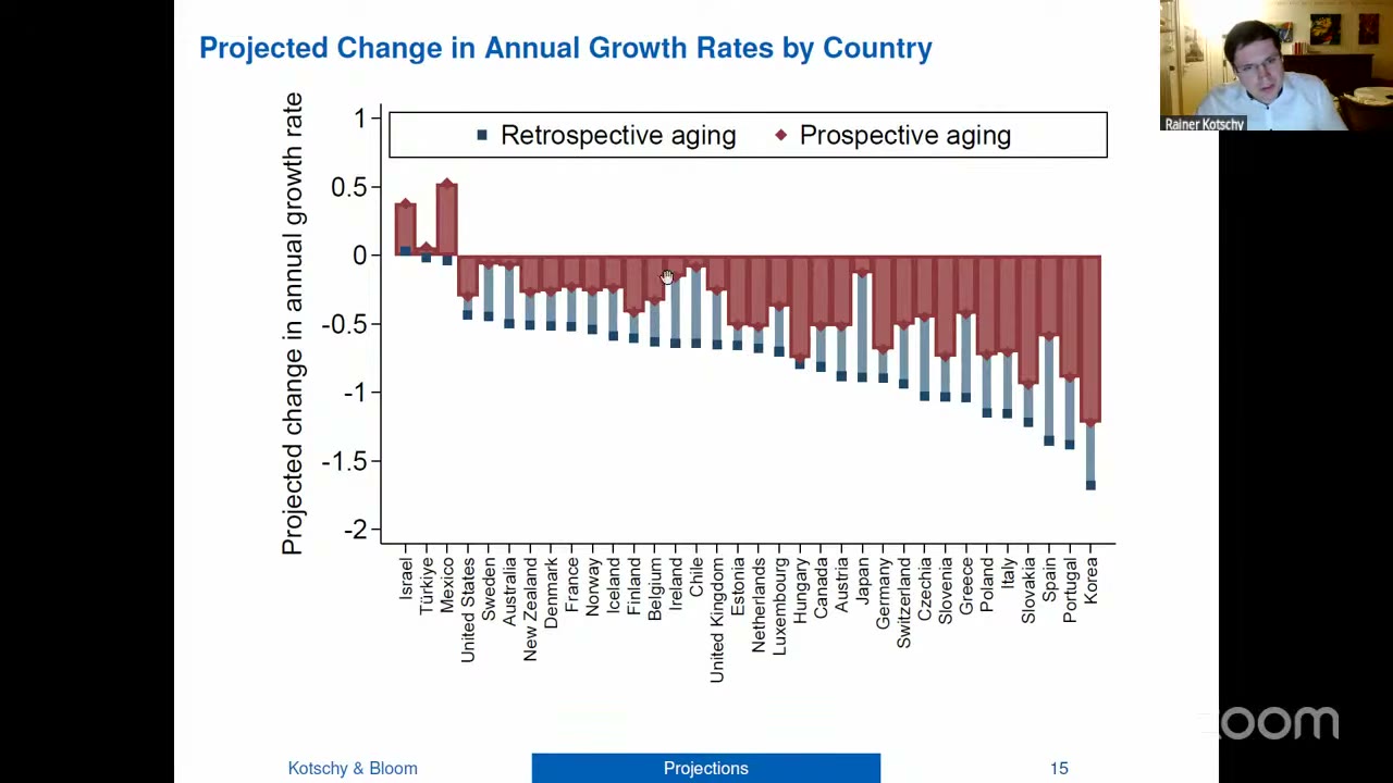
The paper gives three pairs in the text (p. 21). Under retrospective aging, annual growth falls by 0.91 points in Japan, 0.66 in Chile and 0.46 in Sweden. Under prospective aging the declines are 0.13, 0.09 and 0.06. In those countries healthy aging offsets almost all of the drag. In the talk (04:45:08) Kotschy read the retrospective range off the chart, from about 0.4 points in the U.S. to 1.7 in Korea. Those two numbers are chart readings, not figures printed in the paper, but the paper’s Figure 5 shows the same bars.

The U.S. is where the paper’s text and its figure disagree. The text says that across the oecd “up to one-half of the demographic drag can be compensated … with projected values for the United States close to this average” (p. 22). In the talk (04:47:19), Kotschy said the offset is “much more muted” in the United States and Hungary, because those populations are relatively unhealthy. Read by eye, the U.S. bars in both the paper’s figure and the slide are about −0.42 and −0.30. That is an offset of roughly a quarter to a third of the drag. The talk’s description fits the chart better than the paper’s sentence does. It’s a small point, but on U.S. health the paper’s own figure is less optimistic than its text.

In non-oecd countries the dividend is still ahead. Growth rises from 3.4 to 3.8 percent, a gain of 0.4 points, under both definitions (pp. 19–20). The two coincide because the average non-oecd poat reaches about 64 only around 2050. At the country level the prospective dividend is often smaller than the retrospective one, because the poat is below 65 (p. 22). So the chronological measure overstates the drag in rich countries and overstates the dividend in poor ones. Kotschy called this the paper’s first contribution (04:50:25). A 1950–1995 fit projected over 2000–2015 gives a non-oecd dividend worth 10 percent of income per capita over those fifteen years, and none for the oecd (p. 17). That is some evidence the model works outside the fitting sample.

Bounds, and which one we’re near

The authors describe the two aging scenarios as bounds, not forecasts (p. 4; talk at 04:47:34). The retrospective scenario assumes none of the health gains turn into work. The prospective scenario assumes all of them do. “In reality we will probably end up somewhere in between.” That’s reasonable, and it also means the headline “health halves the drag” is an upper bound on the offset.

The appendix has some evidence on where between the bounds countries actually fall, and the talk didn’t mention it. Using aggregated hrs and share data, the authors regress two outcomes on the poat (Appendix Table A.12). One is the stated probability of working full time past 62. The other is actual labour-force participation at ages 63–75. The stated probability rises with the threshold. Actual participation does not move. The authors conclude that “other factors, such as labor market conditions for older workers and the institutional environment, limit the extent to which economic activity extends into older ages.” Here is my reading, not theirs: people report that they could work longer, and so far they don’t. That puts current outcomes closer to the retrospective bound.

What the room pushed on

There was no discussant. The questions mostly went after one choice. The poat moves only the end of working life, and it treats everyone below the threshold as one uniform worker.

The chair, speaking “as organizer” and later addressed as “Adrian” (presumably Adrien Auclert), asked the obvious extension (04:51:38). If health raises productivity at a given age, the effective workforce is the population share at each age weighted by that age’s productivity, and that weighting shifts too. Kotschy agreed the paper is “sort of … a proof of concept” (04:53:11). The measure “focuses really on the mortality margin” and says nothing about age-productivity profiles. He has micro work mapping grip strength into labour supply and non-market activity, but no macro version yet. He would start with one country that has rich microdata. A questioner named “Joe” in the captions pushed further (05:01:59): with productivity gains at every age, or jobs moving away from physically punishing work, could the result go beyond the prospective bound? The honest answer (05:06:15) was that a productivity schedule would give new bounding cases, “no trivial comparison” to the ones shown. So the upper bound holds only within this framework, where the only thing health changes is the age of exit.

“Diego,” who said he was from the World Bank, raised the opposite problem (04:54:36). In low- and middle-income countries older people already “work until you drop,” because there’s no safety net. Development might lower participation at older ages. Kotschy’s answer (04:56:23) conceded most of it: the model is “essentially tailored to the oecd countries.” He kept one claim, that the window for a dividend is shorter than chronological measures suggest. He also suggested modelling a formal urban economy and an informal rural one side by side.

“Ron,” presumably Ronald Lee, made a comment more than a question (04:58:07). In the U.S., labour income at older ages has risen far more than participation. The driver is educated, high-earning people choosing to keep working. So normal retirement ages should vary with lifetime earnings. He mentioned Singapore’s near-zero public transfers to the old, and the low measured productivity of today’s older workers in poorer countries. Kotschy agreed (05:04:49) and favoured flexible retirement schedules. He cited his own finding that chronological age drives exit around statutory ages while health problems push people out earlier. His conclusion was that disability insurance and retirement policy are separate problems.

The last questioner (“Will” per the chair, “Bill” per the captions; 05:03:29) asked about the other end and the middle. Youth underemployment, later entry, and demand for paid leave could offset some of the extra years at the top. Kotschy said he did not have a convincing answer (05:06:42). Age 20 as the start of working life is “an assumption,” and gaps over the life cycle aren’t modelled.

The upshot

The paper does its econometrics carefully, and the econometrics says the answer comes from the definition. With controls, the coefficient is one. So the size of the demographic drag depends on the upper age cutoff, and moving that cutoff with remaining life expectancy halves the oecd number. Most of the questions were about who gets to set that cutoff, and the paper’s own appendix gives a partial answer. People say they would work longer when they’re healthier. Participation data suggest that so far, labour markets and pension systems still mostly treat 65 as the end of working life.

References