Technological Diversification

Miklós Koren and Silvana Tenreyro. Published in the American Economic Review, February 2013 (vol. 103, no. 1, pp. 378–414). pdf-only digest: no talk or discussant was found. Version used: the published aer version plus the online appendix.

Koren and Tenreyro’s “Technological Diversification” is an answer to one of the oldest observations in growth economics, which they take from Lucas: rich countries grow at boringly steady rates, and poor countries lurch. The usual explanations for the lurching are about finance (poor countries can’t insure), about composition (poor countries make a few volatile things), or about policy (poor countries have worse governments). This paper’s explanation is none of those. It is that poor countries run on fewer inputs, and an economy that runs on fewer inputs has fewer things standing between it and any single one of them breaking.

That sounds like a platitude, and in one direction it is. The interesting part is the other direction: nobody in the model is trying to diversify anything. The stability of rich economies falls out of a Romer (1990) expanding-variety model once you let varieties die, with risk-neutral firms who buy new inputs purely because inputs make them more productive. The insurance is a by-product (the abstract’s word) of chasing profits.

The fact being explained is this one. Take non-overlapping decades from 1960 to 2007, compute each country’s standard deviation of annual gdp-per-capita growth, and regress its log on log average income:

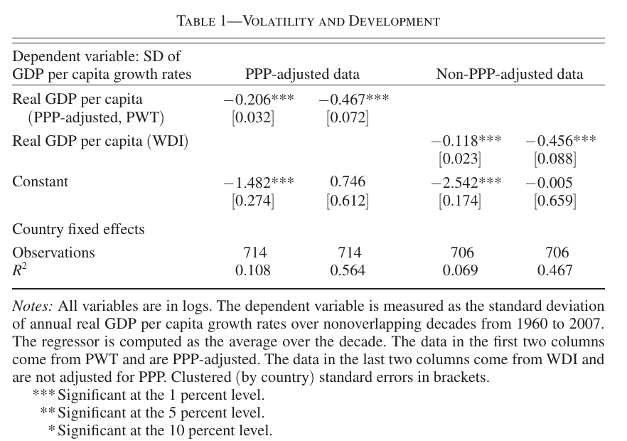
The pooled slope on the ppp data is −0.206, and within countries it roughly doubles to −0.467, so countries get calmer as they get richer, not just rich countries being calm. (One printing quirk: the table’s “Country fixed effects” row is blank; the text tells you columns 2 and 4 are the fixed-effects ones.)

The model

You are a firm. You make your good out of a ces bundle of input varieties (the paper calls them technologies, and means it broadly: a fertiliser, a machine, a kind of know-how). Each variety works perfectly until a Poisson shock at rate $\gamma$ kills it, at which point its productivity goes to zero. Labour moves freely across your surviving varieties, so with $n$ working varieties you produce $A\,l\,n^{1/(\varepsilon-1)}$: more varieties, more output per worker, which is just love of variety. It is also a diversified portfolio. Losing one of your $n$ varieties costs you a fraction of output that shrinks as $n$ grows, and you shift the workers onto the survivors. Your sales-growth variance is $(\lambda+\gamma)/n$ (eq. 29 in the paper): each variety contributes some noise from random adoption and random failure, and you average over $n$ of them. That’s the firm-level story, and it is mechanical.

The aggregate story is where the model earns its keep, and it turns on one asymmetry. Adoption is idiosyncratic: whether your next variety arrives this year is your own coin flip, and across a continuum of firms those coin flips sum to a smooth drift. Failure is common: when variety $k$ dies, it dies for every firm that uses it, all at once. The upside diversifies away in the aggregate, and the downside does not. So aggregate volatility is not about how many firms there are. It is about how concentrated the economy’s usage is across varieties:

Here $N$ is total variety-uses in the economy (gdp is linear in it), $M_k$ is the mass of firms using variety $k$, $s_k$ is variety $k$’s share of all uses, and $\gamma$ is the failure rate, so the right-hand side is the failure rate times a Herfindahl index of technologies (eq. 32 in the paper). If every firm uses a single variety, the index is 1 and the economy has all of $\gamma$’s risk. If every firm uses the same $N$ varieties, it is $1/N$ and the standard deviation falls like $1/\sqrt{N}$. Poor countries are volatile, in this telling, because they have both few varieties and lopsided use of the ones they have: a lot of firms leaning on variety 1. The paper’s illustrations are the nineteenth-century guano crisis, which hit hardest where farmers had no other fertilisers, and the 1993 Sumitomo explosion that wiped out two-thirds of the world’s high-grade chip-sealing epoxy, which it also tells.

The same asymmetry buys a second prediction for free. If gains arrive smoothly and losses arrive in lumps, aggregate growth should be negatively skewed, and in the data about 70 percent of countries do show negative skewness.

The one surprising thing

Now ask how much diversification firms buy. A size-$n$ firm spends $g(\lambda)Ln$ to get its next variety at Poisson rate $\lambda n$, and it sets the marginal cost equal to the jump in firm value from one more variety. Free entry pins the value of a variety at a constant, and the first-order condition collapses:

Here $g$ is the convex adoption-cost function, $L$ the labour force, $V$ firm value as a function of size $n$ and the aggregate firm-size distribution $\mathcal{M}$, and $\kappa L$ and $\eta$ the entrant’s flow cost and success rate, so free entry makes each variety worth $\kappa L/\eta$ (eqs. 14 and 21 in the paper). Read what’s missing from eq. 21. The adoption rate does not depend on $n$, on which varieties the firm has, on how many other firms use them, or on the failure rate. Every firm adopts at the same constant $\lambda$ forever. Nobody in this economy looks at the concentration index, and nobody pays for it. Diversification is a free rider on productivity growth, and the decline in volatility is, as the authors put it, “a by-product of firms’ incentives to increase profits.”

The corollary is the sting. Because nobody prices concentration, nothing guarantees that growth lowers it. Proposition 5 says a marginal increase in the mass of firms using variety $k$, all else equal, raises output and lowers aggregate variance only if $s_k$ is below $\sum_i s_i^2$. Growth into a thinly used frontier variety passes that test, and since the frontier is always thin, that’s the usual case. But if lots of firms pile into a variety that is already everywhere, output and volatility rise together. The appendix gives a worked example where it happens, from $0.272\gamma$ to $0.273\gamma$, which is a small number but the right sign for the point. The paper is candid that the relation is “suitable to explain” the data rather than guaranteed by it, and that in “virtually all” its numerical experiments development and volatility do move in opposite directions.

(A cousin of the same point: for a given $N$, and treating each variety as usable by at most a unit mass of firms, the most volatile arrangement is everyone using the same narrow menu of $N$ varieties. Uniform use of a narrow menu is the most concentrated arrangement there is, however many firms share it.)

The evidence

The firm-level fact comes from Compustat: bigger us firms have less volatile sales growth, whether size is measured by employees or by sales, with and without firm fixed effects.

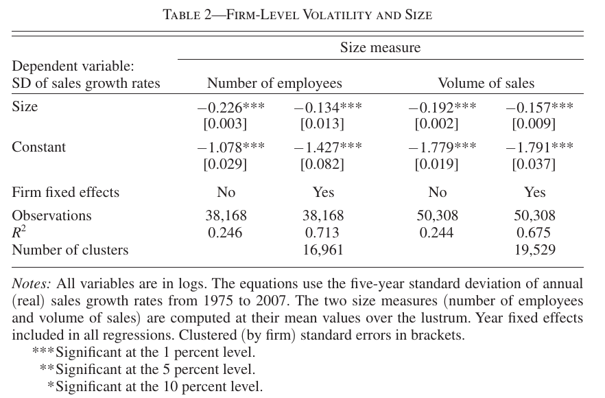
The slopes run from −0.134 to −0.226. The appendix finds the same negative relation in 17 other countries and, importantly for the rival story, among single-segment firms, so it isn’t that big firms simply sell more products. Here is the first place the model overshoots. Since the model’s firm standard deviation is $\sqrt{(\lambda+\gamma)/n}$, its size slope is mechanically −0.5 against the data’s 0.1 to 0.3 in absolute value, and the authors leave closing that gap (heterogeneous intensity of use) to future work.

The third fact is that firm and aggregate volatility co-move positively. Financial-diversification models predict the opposite: firms take more risk as finance deepens, while the aggregate calms down. The paper’s claim is specifically about privately owned firms. The us Great Moderation was, in its words, “overwhelmingly driven by the decline in volatility of nonlisted firms,” while listed us firms got more volatile over the same years, which the authors set aside because listed firms are a small slice of all firms. Note that this means the Compustat firms in the table above are not the population behind the co-movement fact.

Then the calibration. Sixty-four countries with Maddison gdp for 1870 are started from a logarithmic firm-size distribution fitted to their 1870 income, simulated 1,000 times to 2007, and the last 48 years compared with the data. Long-run growth is set at 2 percent, so $\lambda=\gamma+0.02$, $\varepsilon=3$, $\eta=0.1$ from a seven-year median age of nonemployer firms. The failure rate $\gamma$ is not identified, so they run a grid:

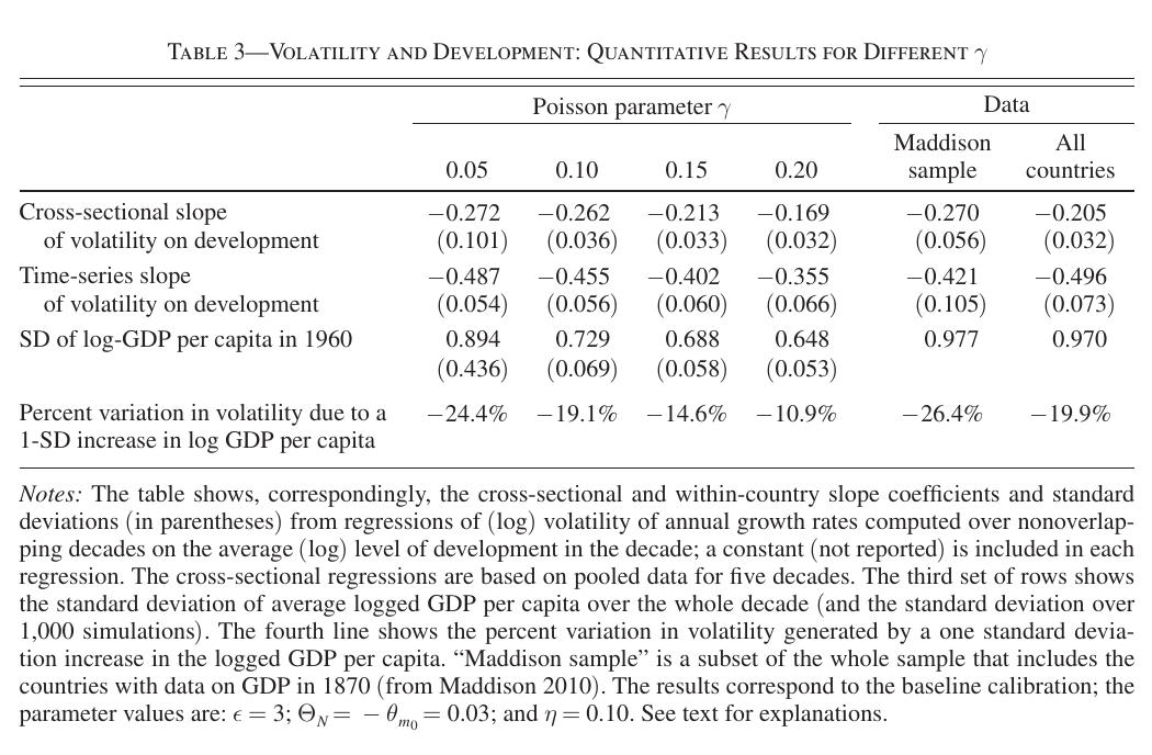
At the “natural” $\gamma=0.10$ (a ten-year average technology life), a one-standard-deviation rise in log income lowers volatility by 19.1 percent in the model against 26.4 percent in the Maddison data. That ratio is the paper’s headline, the model accounting for “around 73 percent” of the variation. Two footnotes on the headline. The 73 percent is measured against the Maddison sample; against the all-countries column it would be higher, a ratio the paper does not state. And the all-countries time-series entry does not match column 2 of Table 1, although the text says it corresponds to it. It matches an appendix regression with a slightly different sample instead. Neither changes the story, but the second is the kind of thing you’d want to know before citing the table.

The model does less well on the third moment. Simulated skewness runs from −0.285 at $\gamma=0.05$ to −0.076 at $\gamma=0.20$, against −0.390 in the data. The authors say the model “could yield higher skewness if negative shocks were not independent across varieties,” which is a suggestion, not a result. And the whole quantitative exercise leans on $\gamma$: the appendix calls it “the most important dimension along which the results vary,” while $\varepsilon$, $\eta$ and the externalities barely matter over the grid it reports.

Objections the paper itself anticipates

(These are the authors’ own pre-emptions; there was no discussant.) On sectoral composition, including their own 2007 paper, they note that within-sector declines are at least as important and that the firm facts hold for single-segment firms. On finance, the volatility–development slope holds within every quartile of financial depth, credit loses significance once other controls enter, and in an appendix extension with risk-averse, credit-constrained firms adoption stays positive, provided adoption costs satisfy Inada conditions. Policy, openness, war, government size and terms-of-trade volatility are controlled for. The all-or-nothing shocks and substitutable inputs are relaxed in the appendix, where a complements version still has volatility falling in $n$ unless shocks are very large. The balanced-growth externalities are declared a convenience, and turning them off at $\varepsilon=2$ reproduces the table.

What they concede is the list above: a firm slope too steep, skewness too mild, too little cross-country income dispersion (the model has no convergence force), and a key parameter they cannot pin down. That’s an honest ledger for a model whose whole engine is one line of algebra about Herfindahl indexes. The nice thing about the paper is that the calm of rich countries turns out to need no one’s prudence. It just needs enough things to break that no one of them matters, and a free-entry condition that stops anyone caring which.

References