Left Behind: Creative Destruction, Inequality, and the Stock Market

Leonid Kogan, Dimitris Papanikolaou and Noah Stoffman, Journal of Political Economy 128(3) (2020), pp. 855–906. Published version, with the 2018 online appendix and the authors’ 2020 erratum. Talk: a segment of Papanikolaou’s 2022 Macro Finance Society summer-school lecture “Innovation and Asset Prices” (no discussant; audience questions interleaved).

Kogan, Papanikolaou and Stoffman’s “Left Behind” is a paper about why a good technology shock can be a bad state of the world for the people who own the stock market. The usual production-based asset pricing story has one household eat whatever the economy makes, so the sign of the price of a technology shock is a fight between the elasticity of intertemporal substitution and risk aversion, and nobody else is in the room. This paper puts someone else in the room. Most of the value of a new idea goes to the person who had it, she could not have sold you a claim on it in advance, and you mind, because you care about your consumption relative to hers. So when the technology frontier jumps, output, investment, wages and eventually your own consumption all go up, and you feel worse. Growth stocks are the assets that pay off in exactly that state. That makes them insurance, and insurance earns a low return, and the value premium falls out.

The recategorization the paper is selling, and it is a real one, is this: the value premium is not a premium for bearing recession risk. It is a premium for holding the assets that lose when somebody else gets rich. Papanikolaou’s own version in the lecture is that you only need a small part of the population to benefit directly from new projects, and then, “if people have some fomo”, they “get upset that other people got rich” (01:08:48).

The mechanism: two technology shocks and one missing market

Production is a vintage-capital economy in the tradition of Solow’s (1960) model. Each project $j$ produces with its own capital and with labor hired at a common wage:

This is eq. (1) in the paper: $u_{j,t}$ is mean-reverting project productivity, $\xi_{\tau(j)}$ the embodied technology level frozen at the project’s creation date $\tau(j)$, $K_{j,t}$ project capital, $x_t$ labor-augmenting technology common to every vintage, $L_{j,t}$ labor, and $\phi$ the capital exponent, which applies to the whole bundle $u\,e^{\xi}K$, not to $K$ alone.

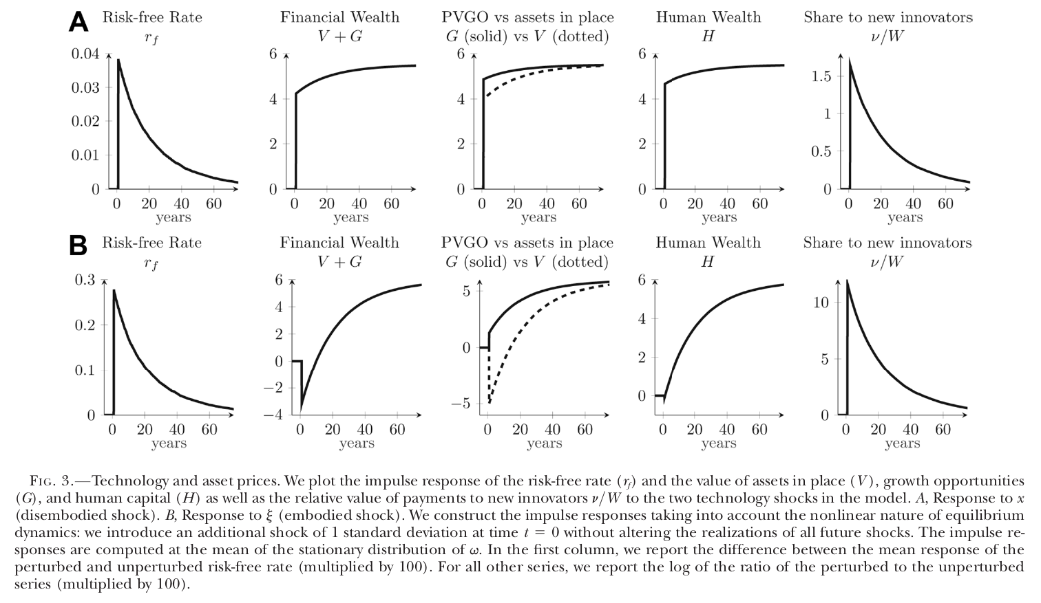
There are two random walks here and they do very different things. A rise in $x$ lifts every project, old and new, and is the textbook productivity shock. A rise in $\xi$ lifts only projects started from now on. Old projects keep the $\xi$ they were born with, and they now compete for the same workers as better new ones. Labor is perfectly mobile across vintages, so the new projects bid up the wage and profits on installed capital fall. That is creative destruction among firms, and it is why, after a $\xi$ shock, the value of assets in place falls on impact while the value of growth opportunities rises (Fig. 3B).

New projects come from blueprints. Households have the ideas, at an idiosyncratic Poisson rate $\mu_I$, and sell them to firms, which supply the investment goods. The inventor keeps a share $\eta$ of the project’s net present value $\nu_t$, and the buying firm’s shareholders get the rest. And then the one sentence on which everything rests: households “cannot trade in securities contingent on future successful individual innovation” (p. 866). Every other market is complete, including annuities in the Blanchard (1985) style and claims on labor income. The friction is not a financing constraint on firms. It is that you cannot sell, today, a share in the idea you might have in 2031.

The size of the lottery you are not allowed to diversify is $\nu_t$ relative to total wealth $W_t$, and that ratio is far more sensitive to $\xi$ than to $x$: in Fig. 3 it jumps by about 12 (×100 log units) after a one-standard-deviation $\xi$ shock and about 1.7 after an $x$ shock. So an embodied shock is a moment when a lot of new wealth is being handed out, by lottery, to people who are not you.

The wealth-share law makes this precise. The published version printed a drift of $\delta^h\,dt$. The 2020 erratum corrects it, because newborn households arrive with only human wealth while existing households hold a mix of financial and human wealth:

This is eq. (27) as corrected by the 2020 erratum (erratum eq. 1, full participation): $w_{i,t}=W_{i,t}/W_t$ is household $i$’s wealth share, $\delta^h$ the death rate, $H$, $V$ and $G$ human wealth, assets in place and growth opportunities, $\lambda$ the aggregate flow of new projects, and $N^I_{i,t}$ the household’s own count of blueprints, arriving at rate $\mu_I$.

Read the second term the way you’d read a fee. Every instant, every household pays $\lambda\eta\nu_t/W_t$ of its wealth share into a pot, and the pot goes to whoever happens to innovate. The jump is symmetric in expectation, so for the household that pays and does not win, which is almost every household, the share drifts down; for the rare winner it jumps. The bigger $\nu/W$, the bigger the fee. This is Constantinides and Duffie (1996) idiosyncratic risk whose size moves with the aggregate state, except that here the state is endogenous: it is the innovation rate itself.

The paper is careful to make this tractable. The measure of blueprints a household gets, conditional on innovating, is proportional to its wealth, so with homothetic preferences every household solves the same problem scaled by $w_i$, consumes $C_{i,t}=w_{i,t}C_t$, and the wealth distribution drops out as a state variable. Papanikolaou in the lecture: the distributions “constantly evolve and respond to the shocks” but “don’t matter for equilibrium prices” (01:20:26). The authors argue in footnote 8 that this assumption probably weakens their result rather than driving it.

None of this would move prices if households only cared about their own consumption, because their own consumption still goes up. So preferences carry the wedge. Households have Duffie–Epstein (1992) recursive utility over a bundle that includes consumption relative to the average:

This is eq. (14) in the paper: $J$ is continuation utility, $\bar C=\int_0^1 C_{i,t}\,di$ aggregate consumption (eq. 15), $h$ the weight on relative consumption, $\gamma$ relative risk aversion, $\theta$ the elasticity of intertemporal substitution and $\rho$ the effective discount rate including mortality.

Because $C_i = w_i C$, the bundle is just $C^{1-h}w_i^{h}$: aggregate consumption to the power $1-h$, your wealth share to the power $h$. The relative concern is proportional, so, as Papanikolaou put it, it “won’t change the coefficient of relative risk aversion” (01:11:35). His microfoundation is competition for scarce local goods: everyone on Wall Street gets a bonus and you are renting, or competing for schools (01:12:02).

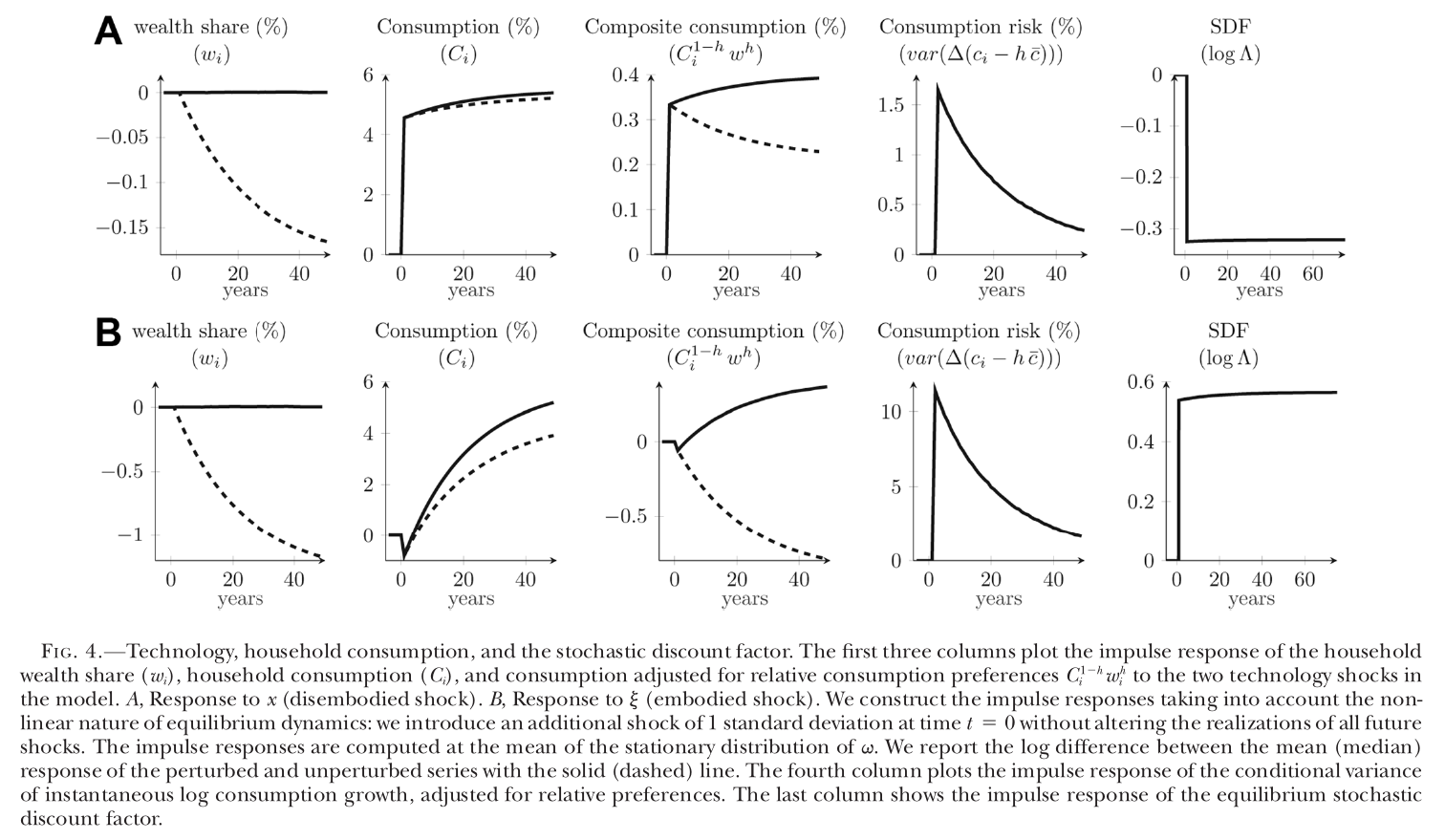
Now run the $\xi$ shock through it, at the estimated parameters, and Fig. 4B is the whole paper in five panels. The median household’s wealth share falls steadily (about one percent of itself over forty years). Its own consumption dips on impact, as investment crowds it out, and then rises. Its composite consumption $C^{1-h}w^{h}$ falls and keeps falling. Conditional consumption risk jumps by about 11 (in the figure’s percent units), and the log stochastic discount factor jumps up by about 0.55. Run the $x$ shock and the sdf falls by about 0.33 instead. The appendix’s risk prices at the baseline are $+0.027$ for $x$ and $-0.078$ for $\xi$. Same sort of good news, opposite sign.

The published text says the mean wealth share is unchanged by either shock at every horizon while the median falls. That is a property of the published drift. With the erratum’s drift, $H/W$ rises after a $\xi$ shock (labor works with any vintage, so human wealth gains), and existing households’ expected relative-wealth growth falls too, which the erratum calls a further displacement channel. So the clean “mean flat, median down” picture is now only approximately right, which if anything helps the paper.

The firm side then writes itself. A growth firm in the model is one with a high arrival rate of new projects relative to its installed size, and a value firm is the opposite.

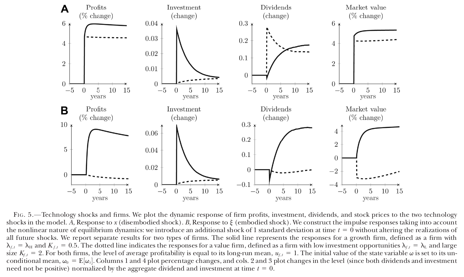
After $\xi$, the growth firm invests and appreciates, and the value firm’s profits fall by about one percent and its market value by about three (Fig. 5B). After $x$, both rise. So growth firms pay off exactly when marginal utility is high, investors hold them as a hedge against being left behind, and they earn less. In the model’s own structural exposures (Table A.2, baseline), the value-minus-growth portfolio loads $-0.875$ on $\xi$ and the market $-0.653$.

This also delivers the paper’s second target, the failure of the consumption capm and the capm. What prices $\xi$ is the dispersion of consumption, not its aggregate. Aggregate consumption dips and then rises after $\xi$, so it is a poor measure of the bad state. And the market portfolio loads on $x$ and $\xi$ in different proportions from the value factor, so it is a poor proxy for the priced shock vector, which leaves a capm alpha on value.

The evidence

The quantitative work is simulated minimum distance: 19 parameters estimated, plus a death rate of $1/40$ and $\mu_I=0.13\%$ calibrated, with equity returns levered 2.5 times ex post because the model has no debt.

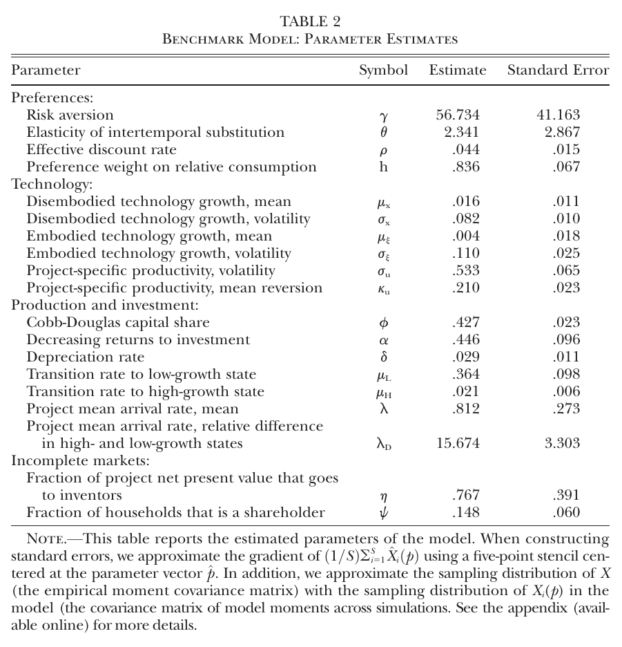
Table 2 is where you should slow down. Relative risk aversion $\gamma$ is 56.7 with a standard error of 41.2. The eis is 2.34. The relative-consumption weight $h$ is .836 (s.e. .067), which means households put most of their utility weight on keeping up. The inventor’s share $\eta$ is .767 (s.e. .391), which the authors translate as “approximately one-fourth” of the value of new investment opportunities accruing to shareholders (p. 888). Only $\psi=.148$ of households hold stocks. (Smaller things: the text rounds $h$ to “approximately 80%”, and the lecture says risk aversion of 40, which does not match Table 2; I quote the table.)

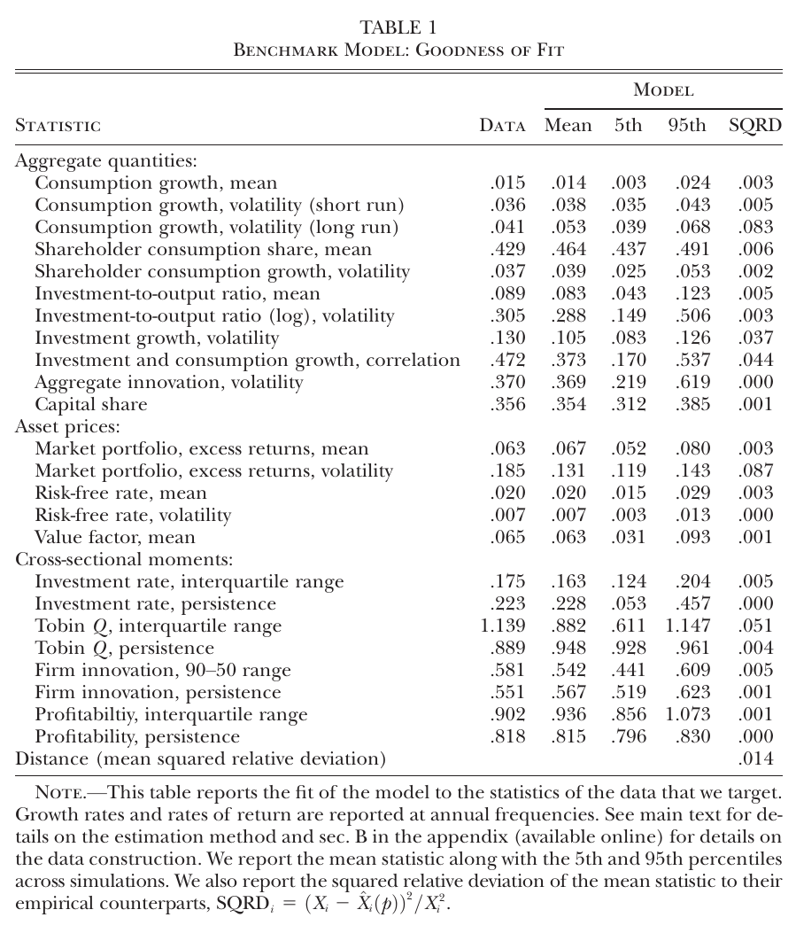
At those parameters the fit is good. From the published Table 1: equity premium .067 in the model against .063 in the data, risk-free rate .020 against .020 with volatility .007 against .007, value-factor mean .063 against .065, consumption growth .014 against .015. Market volatility is the visible miss: .131 against .185, about 30% too smooth. The Tobin’s Q dispersion is the largest cross-sectional miss.

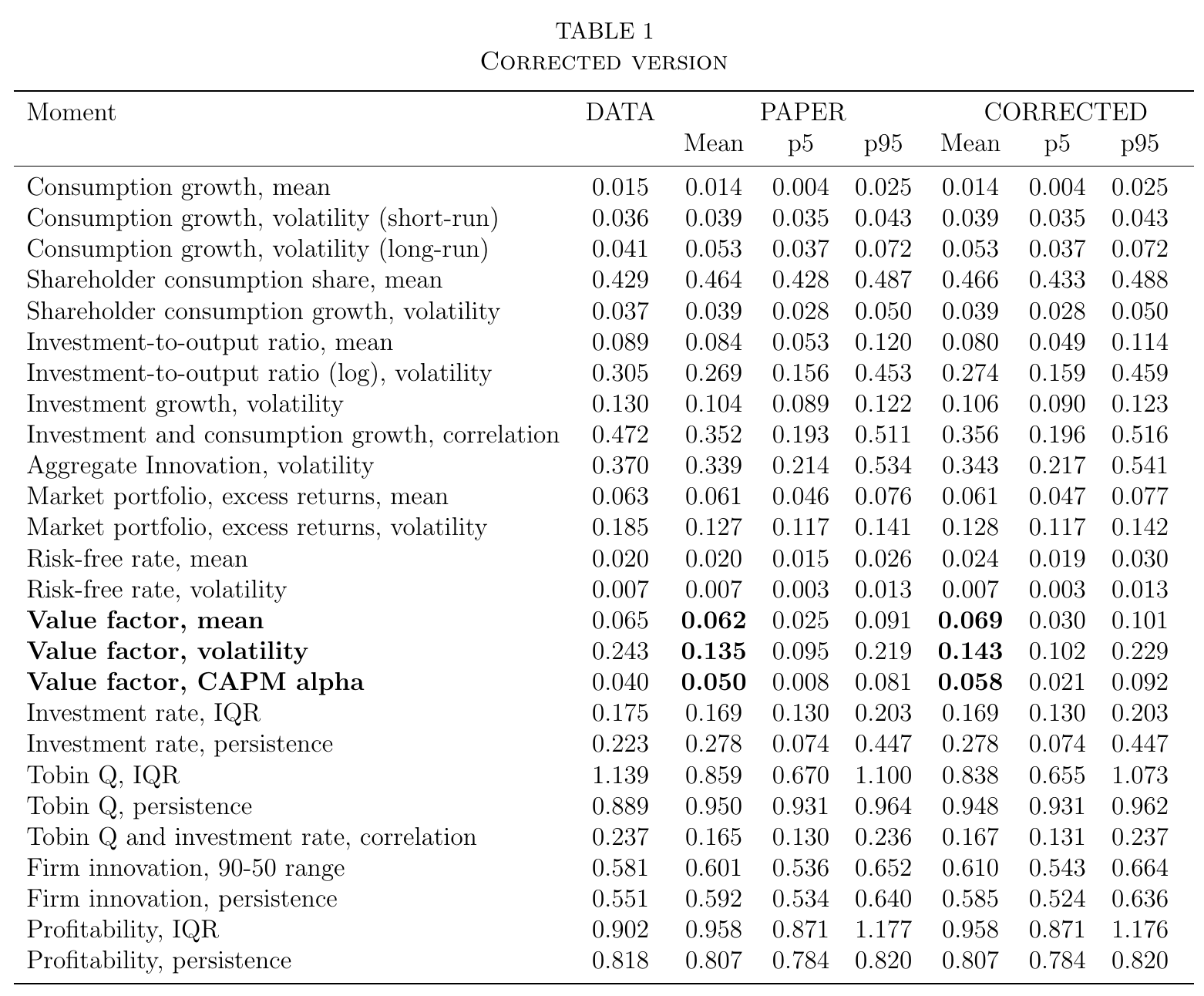
The erratum re-simulates at the same point estimates with the corrected drift. In its “corrected” column the value factor mean rises to .069 (data .065), its capm alpha to .058 (data .040), and the risk-free rate drifts to .024 (data .020). The erratum calls the differences “quantitatively minor and certainly within the bounds of simulation noise”, and that is fair for most rows. But note that the erratum’s “paper” column is itself a fresh simulation and does not reproduce the published Table 1 (market premium .061 there, .067 in the published table), and the erratum’s text quotes the published value premium as 6.2% where the published table prints .063. So I keep the two versions apart: the published Table 1 for the overall fit, the erratum-corrected column for the value moments. Figures 3–5 and 7 and Tables 3–9 were not recomputed; everything else in this note comes from the pre-erratum model.

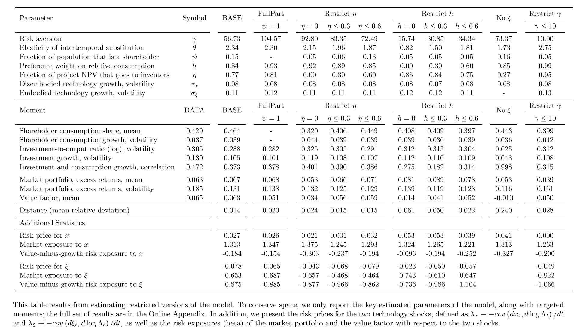
The online appendix’s Table A.2 is the paper’s argument that all three ingredients are needed: embodied shocks, $\eta>0$, $h>0$. Each is switched off and the rest re-estimated. With $h=0$, the value premium falls to .014, the market premium overshoots at .081, and the distance rises from .014 to .061. With $\eta=0$, the value premium is .034 and risk aversion climbs to 92.8. Without $\xi$, the value premium turns negative (−.010) and the distance is .240. These are shown by re-estimation, so they are conditional on the rest of the structure; they say “this model needs all three”, not “the world does”.

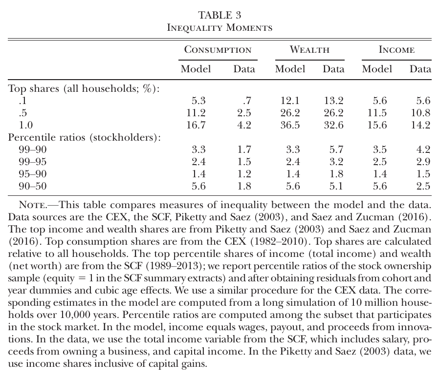
Inequality comes out as a byproduct, and the authors claim this is “the first general equilibrium asset pricing model that can generate realistic patterns of inequality” (p. 891). Top 1% wealth share: 36.5% in the model, 32.6% in the data. Top income shares match closely too, but with an asterisk. The innovation rate $\mu_I$ is calibrated to top income shares; pp. 884 and 891 and the online appendix say it is the top 1% share, and p. 890 says top 0.1%. Either way, the income rows are at least partly targeted. The consumption row is the miss: the model’s top 1% consumes 16.7% of the total against 4.2% in the cex, which undersamples the rich, but not by that much.

Then the direct tests. The paper builds a model-consistent innovation measure: a nonparametric approximation to the patent-value method of Kogan et al. (2017), which takes the positive part of a firm’s three-day market-adjusted return around each patent grant, times its market cap, split across same-day grants, and scales the sum by total market value. The same construction is run on simulated data, which is the nice part: the data moments and the model moments are measured the same way.

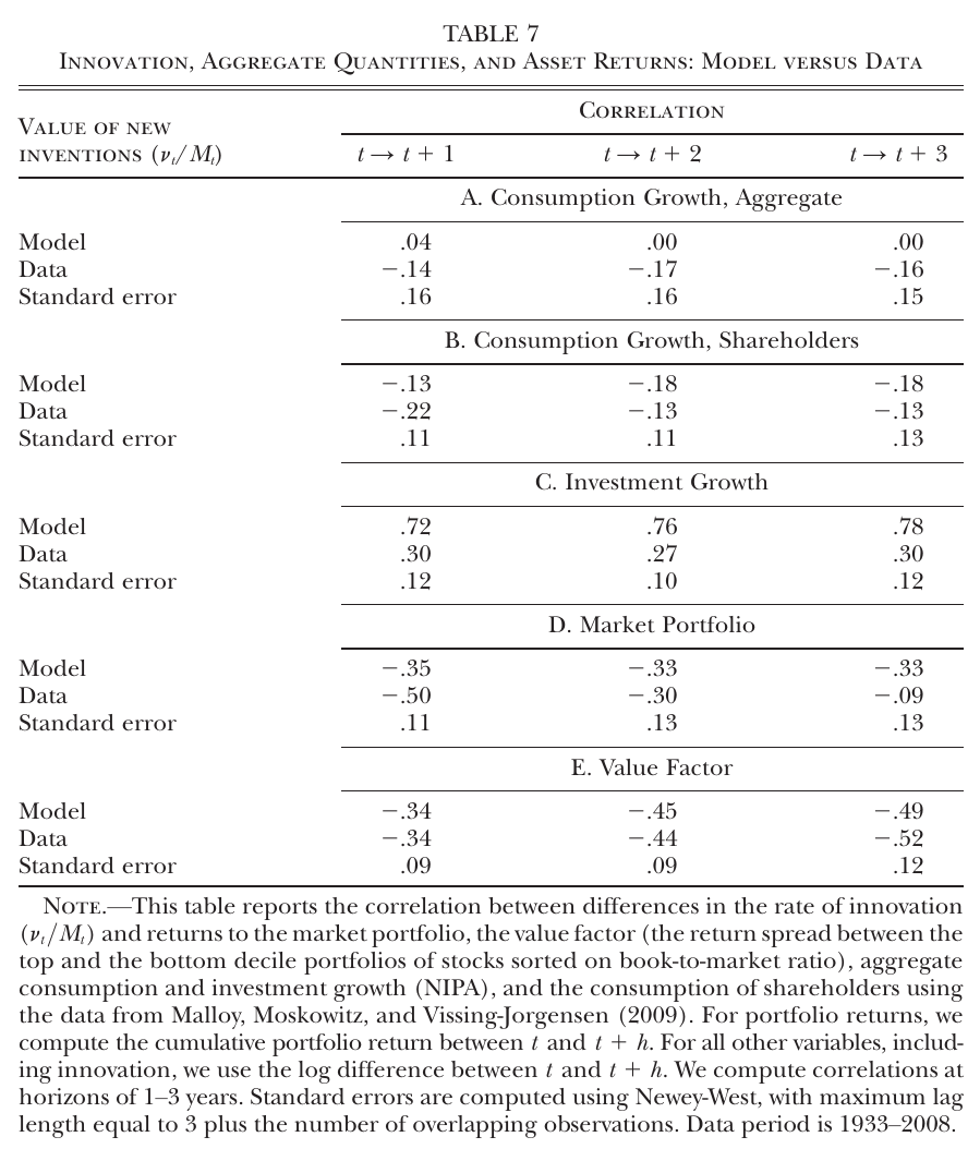
Table 7 correlates log changes in that measure, over one to three years, with growth rates and cumulative returns. The value-factor row is uncanny: −.34, −.45, −.49 in the model against −.34, −.44, −.52 in the data. The market row is negative in both. Investment is too tightly linked in the model (.72 to .78 against .27 to .30; the text’s “60%–66%” for the model does not match the table). Aggregate consumption is roughly uncorrelated in the model and mildly negative in the data, with standard errors of .15 or so, and the shareholder-consumption row uses the Malloy, Moskowitz and Vissing-Jorgensen (2009) series, which covers only 1982–2002 within the table’s 1933–2008 window.

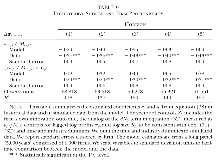
Table 9 is the firm-level displacement test and the most direct one. When a firm’s industry rivals innovate (one standard deviation of the leave-one-out measure), a value firm’s profit growth falls by .037 to .043 standard deviations over one to five years in the data, against .029 to .069 in the model, all significant at 1%. The growth-firm interaction is positive, .024 to .031 in the data, which means growth firms are hurt less, not that they gain. The model matches at one to three years and becomes too heterogeneous at longer horizons, which the authors attribute to the absence of firm exit and to small growth firms missing from Compustat. (The text says horizons one to six; the table has five columns.)

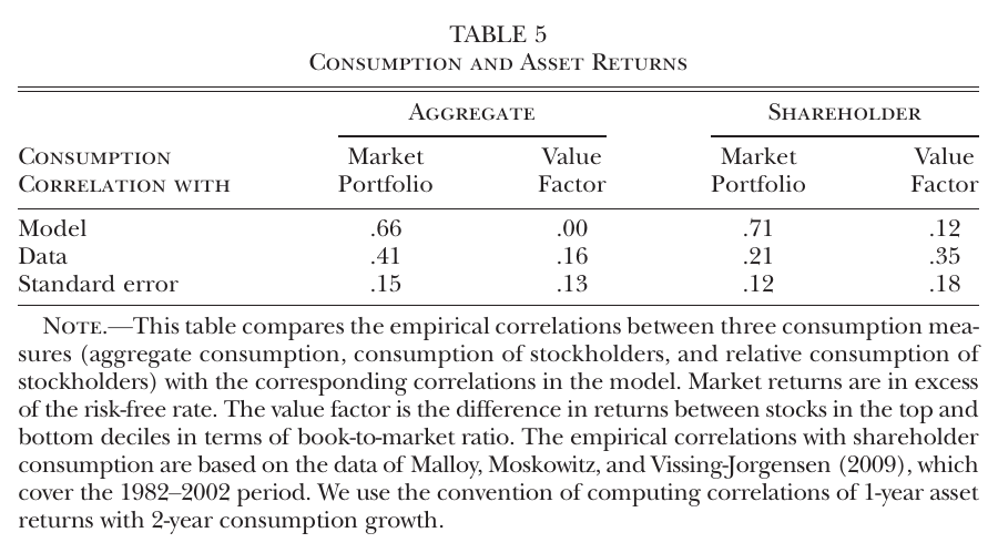
And the consumption-capm evidence is Table 5: in simulated data the value factor’s correlation with aggregate consumption growth is .00 (data .16). The value premium is priced, and aggregate consumption does not see it. The miss here is the market’s correlation with shareholder consumption, .71 in the model against .21 in the data, which the authors acknowledge.

The one surprising thing

It is not that good technology news can raise marginal utility. Papanikolaou spends the first minutes of the segment explaining that a representative-agent model can deliver either sign: on impact investment rises and consumption falls, so a time-separable household’s sdf rises, and with recursive utility the sign then depends on the eis against the reciprocal of risk aversion (01:09:15). Here the eis is 2.34, so that representative household would cheer.

The surprising thing is how the paper gets risk aversion of 57 to mean almost nothing about aggregate risk. The appendix’s projected sdf loads on the stochastic trend $\chi_t$ with an effective coefficient $\gamma_1 = 1-(1-\gamma)(1-h)$. With $h$ near one, $\gamma_1$ collapses. My arithmetic at the point estimates (not in the paper): $\gamma_1 \approx 1 + 55.73\times 0.164 \approx 10.1$. So the headline $\gamma$ overstates how much these households fear aggregate shocks by a factor of five or so, and almost all of what is left over is fear of falling behind. That is also why $h$ is identified by the gap between the market and value premia: a higher $h$ lowers the equity premium and raises the value premium. Push it to the limit in the $\gamma\le 10$ re-estimation and $h$ goes to .99, the price of $x$ goes to zero, and, in the appendix’s words, households “care almost exclusively about displacement risk”. The model still produces a value premium of .050 there. So the paper is, at bottom, an asset pricing model in which the representative agent’s main concern is the neighbours, and the remarkable thing is how many standard moments that one concern buys.

What the lecture audience pushed on

There was no discussant; the questions came from a summer-school audience, mostly by chat, and I paraphrase them.

One participant asked whether the sdf result just means people save more when a great innovation arrives because the future looks better. Papanikolaou’s answer, as I understand it, was no: the risk-free asset is in zero net supply, so the economy can only save by investing, and $\xi$ is not manna, it pays off only if resources are given up now. The trade of less now for more later is the robust part, and “what’s not robust is how you feel about it” (01:15:35); in q-theory language, “what’s moving around is marginal q” (01:18:04). The questioner’s cancer-drug example, where the spillover reaches everyone, is useful precisely because it is what the model denies for the financial rents.

Another asked whether all-equity financing matters, since with debt the payouts that fall after $\xi$ would look different. He agreed there are no financial frictions at all, said a fixed debt claim would mechanically amplify equity volatility, and on endogenous capital structure said “these are all interesting questions but I don’t know the answer” (01:30:32). A related clarification: “dividends” in the model are free cash flow, profits minus investment, so the model makes no dividend-policy predictions (01:23:30).

A third asked why the sdf response is so permanent. His answer was that risk premia are roughly constant and the risk-free rate barely moves, so the sdf has a large permanent component, the property Alvarez and Jermann (2005) say is needed to rationalize an equity premium over long bonds. The risk-free rate is stable because the precautionary effect of more idiosyncratic risk and the growth effect offset, and because low rate volatility was a target. Asked himself whether that is a deep feature: “No” (01:33:11).

He was also his own sharpest critic. After the corrected fit: “the model is a little bit too well relative to the data” (01:36:33), which matches the corrected alpha of .058 against .040. On parameters, risk aversion “which I’m told is too high” and households putting most of their weight on relative consumption: “relatively extreme parameters” (01:38:35). And on labor, which is “a great hedge for technology” in the model (01:39:17): no labor-market frictions, fully diversifiable labor income, no skill displacement, no automation (01:40:10). It is a list of exactly the channels that would make labor a worse hedge, and he presents it as an agenda rather than a defence.

Weak points, my own reading

The identification is thin where the story is thick. The two parameters that carry the mechanism, $\eta$ and $\gamma$, have standard errors of .39 and 41, and $h$’s tight standard error comes from the one moment it is designed to fit.

Tradable, perfectly mobile labor does more than the paper admits in the main text. It makes labor income a $\xi$-hedge for shareholders, it produces the counterfactual 90–50 income ratio in Table 3, and in the appendix it yields a negative price of $\xi$ even with $\eta=0$, because aggregate consumption includes non-participants’ wages, which rise with $\xi$. The authors call both of those effects “an artifact of the stylized nature of our model”. Fair, but it means part of the estimated $\xi$ price is not inventor displacement at all.

Blueprints proportional to wealth is the tractability assumption, and it is argued to be conservative rather than shown to be.

The innovation measure is a stock-market reaction scaled by stock-market value. Correlating it with market and value returns, as Table 7 does, is partly mechanical, and a common discount-rate shock would move both. The industry leave-out in Table 9 handles a firm’s own patents, not that.

Consumption inequality is far too high (16.7% against 4.2%), and that is not a side miss: $C\propto W$ among shareholders is the assumption, and consumption dispersion is the channel through which the sdf moves.

Volatilities are missed across the board (market .131 against .185; value-factor volatility .143 corrected against .243), which weakens the capm-failure story somewhat, since alphas are easier to match when the factor is too smooth.

And the erratum bookkeeping is messier than “quantitatively minor” suggests: the corrected risk-free rate is off target, the erratum’s “paper” column is not the published table, and most of the paper’s figures and tables were not recomputed.

None of the empirical work observes the marginal investor’s innovation-contingent marginal utility. What it shows is that the innovation measure moves value-firm profits, inequality and the value factor in the directions and roughly the magnitudes the model predicts, which is more than most asset pricing models of the value premium can say, and a good deal less than proof.

Still, it is an unusually honest piece of machinery. It takes “creative destruction” literally enough to put the destroyed in the utility function, finds that they set the price of growth stocks, and then has one of its authors tell a room of graduate students that his households are too risk-averse, too envious and too lucky in the labor market. The value premium, on this account, is what you pay to not mind your neighbour’s ipo.

References