Technological Innovation, Intangible Capital, and Asset Prices

Leonid Kogan and Dimitris Papanikolaou, Annual Review of Financial Economics 11 (2019): 221–242, first published online December 2019. Published version; a review article, so no discussant and no recorded talk of it. Papanikolaou’s 2022 Macro Finance Society summer-school lecture, Innovation and Asset Prices, covers much of the same ground and was not used here.

This is a survey, and like most surveys by people who built the field, it is also a map of their own house. Kogan and Papanikolaou spent the 2010s arguing that technological progress is not one shock but two, that the two have opposite effects on the people who own today’s stock market, and that a good deal of the cross-section of returns is the market pricing the difference. The review is their attempt to say that cleanly, and to say what “intangible capital” has to do with it. Its answer to the second question is, roughly, less than you’d think, for the reasons you’d expect, and then a lot more, for a reason you might not.

They start with definitions, and the definitions do real work. Capital investment is any outlay meant to raise future rather than current consumption, following Corrado, Hulten and Sichel (2005). Intangible capital is the accumulable factor with no physical presence: brands, patents, production know-how, organisation capital, human capital. It has two awkward properties. It is mismeasured, so it hides in the gap between output and the inputs you can count. And it is “more than poorly measured capital stock”: the talented division manager who makes the firm more productive is part of its intangible capital, but nobody can quite say which part of the output is hers, so nobody can quite say who owns it. Hold on to that second property; it is where the review ends up.

Technological innovation, meanwhile, is defined as “an outcome that lowers the cost of investing in either physical or intangible capital”. That is a deliberate choice. The usual move in macro is to call innovation a shift in total factor productivity, something that makes the capital you already have more productive. Kogan and Papanikolaou put the action on the investment side instead: innovation makes it cheaper to build new capital, a better computer blueprint, a new drug, a new process. Building a factory is investment but not innovation; finding a cheaper way to build factories is both.

The mechanism, part one: the workhorse models are one model

The first half of the review lays out three workhorses, and its punchline is that they are the same animal. In the neoclassical growth model with convex adjustment costs, capital accumulates as $dK = \chi I\,dt - \delta K\,dt$, the first-order condition is Q theory, and capital grows faster when the market values it more. In Romer (1990)’s expanding-varieties model, R&D creates monopoly licences for new intermediate goods; with the research technology of Comin and Gertler (2006) and Kung and Schmid (2015) plus free entry, the growth of varieties is a function of the market value per variety, which the authors call “the direct analog of the Q theory of investment”. In the quality-ladder models of Grossman and Helpman (1991) and Aghion and Howitt (1992), research improves the leading quality of existing products, and free entry delivers the same form again.

So the three are mathematically equivalent: one accumulable factor, one disembodied productivity shock $Z$, the same aggregate asset prices. Renaming the factor “knowledge” does not produce a new pricing mechanism. What the models share is the thing that matters for asset pricing: a marginal cost of creating capital that is not constant, so Tobin’s Q moves, so expected growth has a slow-moving component, which with Epstein–Zin (1989) preferences is long-run risk in the sense of Bansal and Yaron (2004), with the production-side version in Kaltenbrunner and Lochstoer (2010). Whether “investment” in the model is capex or R&D changes the quantitative mapping to data. It does not change the economics. (The claim is about these specifications, not a theorem about every growth model, and the review does not pretend otherwise.)

This is a slightly deflating result for anyone who opened a review with “intangible capital” in the title hoping to learn that intangibles are special. In the workhorse models, they aren’t.

The mechanism, part two: where the shock lands

What is special is which capital a shock improves. Set the labour share to zero in the neoclassical model and switch to Solow’s vintage capital. Each vintage produces with its own efficiency, output is $Y_t = Z_t K_t$ where $K_t$ is quality-adjusted capital, and capital accumulates as

This is eq. 27 in the paper: $K_t$ is quality-adjusted capital, $I_t$ investment, $\delta$ depreciation, and $\chi_t$ the productivity of the newest vintage, now a moving state, which makes it an investment-specific technology shock.

Compare it with the constant-$\chi$ version and the only change is that one letter now moves. But look at where the two shocks enter. $Z$ multiplies every vintage, so a good $Z$ shock raises output today, and consumption and investment rise with it. $\chi$ touches only what you are about to build. A good $\chi$ shock leaves output unchanged on impact; the return to investing jumps, so investment jumps, so consumption falls for a while, and output catches up only as the better capital gets installed.

You can see where the pricing goes. Papanikolaou (2011) shows that with power utility the investment-shock risk premium is negative: a high-$\chi$ state is one where a marginal unit of wealth is unusually valuable, because it can be turned into unusually productive capital. You would pay to hold an asset that does well in those states. With Epstein–Zin it depends. Low elasticity of substitution and low risk aversion keep the premium negative; high values of both can flip it, because a good $\chi$ shock raises continuation utility and lowers the marginal value of wealth. So “is technology risk priced, and with which sign?” has the honest answer “tell me your preferences first”. The review is clear about this, and it is worth being clear about, because the second half of the review is in part an attempt to get a sign that does not hang on it.

Then there is displacement. New, better capital makes old capital worth less, so if the stock market is mostly a claim on installed capital, good news about future growth can push it down. Greenwood and Jovanovic (1999) and Hobijn and Jovanovic (2001) read the information-technology revolution this way: incumbents’ valuations fell (the review says “in the late 1960s”) because the firms that would profit from the revolution did not exist yet. In the varieties model the same thing appears in one line:

This is eq. 28 in the paper: $\Pi_t$ is the profit of an existing licence, $Z_t$ disembodied productivity, $N_t$ the number of varieties and $\alpha$ the variety exponent in output; when goods are substitutable enough that $\alpha<1$, entry bids up the fixed labour supply and cuts incumbent profits.

Now put firms in. Firms differ in how much of their value is assets in place and how much is growth opportunities. A $Z$ shock has “mostly a symmetric effect” on both; a $\chi$ shock hurts the first and helps the second. Kogan and Papanikolaou (2013, 2014) build firm-level models in which the growth-opportunity share lines up with observable characteristics, and calibrated versions reproduce the value premium and other characteristic patterns. The review is candid about the hinge: they do so “under the assumption that the risk premium associated with ist shocks is negative”. Growth stocks hedge investment shocks; if investment shocks are bad states, growth stocks are insurance, and insurance earns less. That is a coherent story with one free sign in it.

Measurement

The middle of the review is a tour of how people measure the two objects, and it is mostly an inventory of ways to be wrong.

For intangible stocks, the accountant’s route is the perpetual inventory method: accumulate spending, depreciate it. That requires a depreciation rate and a starting stock, and the review notes that the bea’s 15% for R&D may be too low, and that own-account software is imputed on the assumption that programmers and systems analysts spend about 50% of their time writing software. Corrado and Hulten’s growth accounting, as the review reports it, has intangible investment outpacing physical investment over the past 30 years and accounting for about a quarter of the growth in output per hour. At the firm level, people accumulate sg&a into organisation capital, advertising into brand capital, and fold intangibles into Q, as in Peters and Taylor (2017). The method’s quiet assumptions are that vintages are interchangeable and that depreciation means decay, when a production method may be discarded perfectly intact because a better one arrived.

The financial economist’s route is to let prices reveal the stock. Griliches (1981) regressed market value on tangible and R&D stocks; Brynjolfsson, Hitt and Yang (2002) found each $1 of computer capital associated with about $12 of market value, which is either a lot of complementary intangible capital or a lot of something else correlated with computers. Hall (2001) went further and inverted the adjustment-cost first-order condition to back out total capital from market values, concluding that the bulk of late-1990s market value was a large stock of intangibles, and finding “capital disasters” such as 1973–1974. The review adds two caveats that are really one: the inversion reads every move in valuation as a move in quantity, so a change in risk premia (2008–2009, in the review’s example) shows up as capital destroyed; and it assumes shareholders own all the rents from intangibles, so if employees capture some, it can undercount them. Remember that second caveat too.

For innovation itself, patent counts are the obvious measure and a notoriously bad one: values are wildly heterogeneous, mapping patents to industries is hard, and citation weights help less than one would like. Relative prices of equipment give you $1/\chi$ directly, but only with constant returns to investment and correct quality adjustment, and Bils and Klenow (2001) estimate that official prices missed about 60% of quality growth in a sample of 66 durables.

The review’s preferred route is the authors’ own. Pakes (1985), with 120 firms over 1968–1975, found an unexpected patent associated with about $810,000 of market value. Kogan, Papanikolaou, Seru and Stoffman (2017) turn this around and use the stock reaction on the day a patent is granted to value the patent. The reaction is not the value, because the market already expected some chance of a grant; it is the value times the probability the application would have failed, $\Delta V_j = (1-\pi_j)\xi_j$, and the unconditional grant probability in 1991–2001 is about 56%. Filter out the rest of the day’s news, sum the patent values for a firm and scale by its size, and you have a firm-level innovation measure in dollars. These are private values to the patenting firm, which is what an asset-pricing paper wants and not what a welfare paper would.

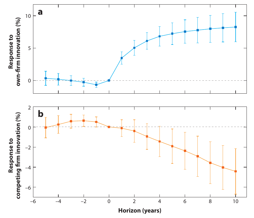
The one new piece of evidence in the review uses that measure. Regress the log of a firm’s average profit over the next $h$ years, relative to its current profit, on its own innovation and on the average innovation of its three-digit sic competitors (leaving the firm out). Two changes from the 2017 paper, averaging future profits and dating patents by application year, do not, the authors say, “substantively affect our findings”. A one-standard-deviation increase in own innovation goes with roughly 8% higher average profits over the next decade. The same increase in competitors’ innovation goes with roughly 5% lower profits. The plotted competitor point at ten years sits nearer $-4.4$, with wide bands that include zero for the first three or four years, so “roughly 5%” is a rounding, not a fib. Pre-period coefficients are small. This is creative destruction at firm scale: your patents raise your profits, your rivals’ patents lower them, and the second effect is slow.

It is worth being exact about what Figure 1 shows. It shows cash flows responding to an innovation measure built from stock returns. It does not show a price of risk, and it does not by itself identify an exogenous technology shock. It is the cash-flow half of the story, and it is a nice picture of it.

The mechanism, part three: who owns the future

Here the second property of intangible capital comes back. Human capital is inalienable, as in Hart and Moore (1994): you can own a share of a firm, but not of the person whose head the firm’s know-how lives in. So some of the cash flow that intangibles and innovation generate never reaches the people holding the securities.

The first version is Eisfeldt and Papanikolaou (2013)’s organisation capital. A firm’s output is $Z_tK_i + Z_te^{\varepsilon_i}X_i$, where $X_i$ is know-how embodied in key employees. Shareholders fully own the physical capital. They only partly own $X_i$, because the employees can leave, buy the physical capital and run a firm at the frontier efficiency $\chi_t$, and the better the frontier, the better their outside option. So a better frontier transfers value from shareholders to talent without making anyone more productive inside the firm, and the shareholders’ claim on intangibles is short the frontier. (The review asserts that this value falls in $\chi_t$; it does not show the sign, which on the printed formula holds only for some parameter values.) In the data, firms with more organisation capital, measured by accumulated sg&a, earn higher risk-adjusted returns, “consistent with a negative risk premium on the frontier technology shock”. That is again a negative premium, and again it is assumed in the model and read off the data.

The second version, and the heart of the review, is general equilibrium, from Kogan, Papanikolaou and Stoffman (2020), in a two-period form taken from Kogan and Papanikolaou (2018). Every period some people, at random, get new ideas: engineers, entrepreneurs, start-up employees, executives, and in the review’s footnote even angel investors and venture capitalists. Nobody can contract today to share the rents from ideas that have not arrived yet. So, in the authors’ phrase, “firm owners reap only part of the benefits, yet all of the costs, of creative destruction”.

The model is small enough to carry in your head. At $t=0$ there is only the old technology, $Y_{o,t}=(X_tL_{o,t})^{1-\alpha}$, and investors with log utility own every firm. At $t=1$ an equal number of new projects arrives, $Y_{n,1}=\chi_1^{\alpha}(X_1L_{n,1})^{1-\alpha}$, where $\chi_1$ is the vintage shock. A fraction $\omega$ of firms get one new project each; the rest go to inventors, who can sell them to existing firms only at fair value, which pays the inventor the rent rather than handing it to the buyer. Workers supply one unit of labour in total and own nothing. Both technologies hire from the same pool at the same wage. (The review’s text calls the labour-augmenting shock $Z_t$ while every equation calls it $X_t$; same object.)

You own the stock market. A wonderful new technology arrives. Output rises. But the new projects bid up the wage, so your old projects earn less, and you own only $\omega$ of the new projects that did the bidding. If $\omega$ is small enough, your consumption falls in the state where the economy got better. Formally,

This is eq. 46 in the paper, with the restriction of eq. 44: $\pi_1/\pi_0$ is the investors’ stochastic discount factor, $C_t$ their consumption, $X_1$ the common labour-augmenting shock, $\chi_1\in(0,\bar\chi)$ the new-vintage shock, $\omega$ the share of new projects incumbents own and $\alpha$ the profit share; under the restriction the discount factor rises in $\chi_1$.

The restriction is assumed, “for simplicity”, not derived; it is what turns the missing market into the right sign. Given it, the asset-pricing results fall out. Claims on new-technology projects pay off in exactly the states investors fear, so they earn less than claims on old projects. Call firms with only old projects value firms, and firms that also own a new project growth firms. Growth firms are priced higher, which is just the extra project, and earn lower expected returns, which is the value premium. Linearise and every firm has the same loading on $X_1$, while growth and value load in opposite directions on $\chi_1$; so growth minus value has no exposure to the ordinary productivity shock and is a mimicking portfolio for innovation. That is the value factor of Fama and French (1993), with an economic interpretation attached.

The one surprising thing

You can own the whole stock market and still not own the future. That is the line the review is building towards, and it is a genuinely different reason for the sign than the one in the first half. In the vintage-capital model, innovation is a bad state only if your preferences make the temporary consumption sacrifice painful enough, and you have to argue about elasticities to get there. In the missing-market model, innovation is a bad state for the people who price stocks because it is a transfer away from them: to workers through the wage, and to inventors through rents nobody could sell in advance. Better technology, poorer shareholders. It comes with log utility, a measure-zero set of inventors, a small enough $\omega$ and, implicitly, two shocks the review never says are independent, but within those it does not need you to pick a corner of the Epstein–Zin parameter space. The value factor becomes compensation for being on the wrong side of creative destruction, which is the sort of interpretation the factor-zoo literature rarely gets offered.

There is a smaller surprise sitting next to it. The review sets out to explain intangible capital and spends its first section showing that, in the standard models, “intangible” does nothing. The label is not the mechanism. Embodiment and ownership are.

Weak points, my own reading (no discussant exists)

The obvious one is that this is a review of a research programme by the people who run it. Nearly every mechanism, and the one new exhibit, comes from the authors’ own papers, and the competing explanations of the value premium do not appear. That is a fair choice for a review that wants to make one argument well, but the reader should know it is one argument.

The sign of the price of innovation risk is assumed in the firm-level models and supplied in the general-equilibrium model only under a bound on $\omega$ that is never quantified. How much of future innovation is really uninsurable for today’s shareholders, given internal R&D, acquisitions and venture exposure, is the question the whole story rests on. The footnote that counts venture capitalists among the “inventors” sits awkwardly here: they are investors with market access, and the more of the rents they capture, the less missing the market is.

The evidence side is thin on prices. Figure 1 is about profits, built from a measure made of stock returns; the only return evidence in the review is the Eisfeldt–Papanikolaou sort on organisation capital, reported without magnitudes. And “intangible equals inalienable human capital” covers organisation capital better than it covers brands, software or patents, which can be sold.

Finally, some printed slips. Eq. 48, the return on old-technology claims, multiplies by $\mathbb{E}_0[(1+\omega\chi_1)^{-1}]$ where pricing with eq. 46 (and the analogous eq. 49) requires dividing by it; the comparative static the authors draw from it is unaffected. The text before eq. 16 cites “Equation 4” where it means eq. 15, and several letters ($X$, $\chi$, $\alpha$) mean different things in different sections, so a reader moving between them should rebind each time. And the review dates the it-driven fall in incumbent valuations to “the late 1960s” while a few pages later linking the 1973–1974 capital disaster to the same revolution.

None of this undoes the point. The review’s real contribution is to say, compactly, that the interesting thing about innovation for asset prices is not that it is intangible but that it is new and that somebody else owns it. Which is also, if you think about it, the standard complaint of every incumbent.

References