Technological Innovation, Resource Allocation, and Growth

Leonid Kogan, Dimitris Papanikolaou, Amit Seru and Noah Stoffman, Quarterly Journal of Economics 132 (2), 2017, 665–712. Read from the May 2016 nber revision (Working Paper 17769), the last public version before publication, with the online appendix; no recorded talk.

Kogan, Papanikolaou, Seru and Stoffman want to measure innovation in dollars, and their measuring instrument is the stock market. The usual instruments are patent counts and citation-weighted patent counts, and both have a units problem. A count tells you that something was invented. A citation tells you that later inventors found it worth mentioning, which is a fine measure of scientific influence and a strange measure of what the patent is worth to the firm that owns it. What a growth economist in the Schumpeterian tradition actually wants is the present value of the monopoly rents the patent confers, since that is the object the theory says firms are chasing and the object whose arrival reshuffles resources between firms. Pakes (1985) and Austin (1993) had already looked for patent news in stock returns. This paper industrialises the idea: about 1.8 million patents granted to public firms over 1926–2010, each with a dollar value read off the owner’s stock price, then summed up to firms, to rivals and to the whole economy.

On 13 November 2001 Amazon was granted a patent on using shopping carts to generate recommendations (the “customers also bought” box), and its stock rose 34 percent in two days, about $900 million of market capitalisation. In the same year ibm was granted a patent on a system that lets airline passengers reserve a place in the queue for the restroom. Its three-day return was slightly negative, and ibm later stopped paying the renewal fees. But it received 21 citations, which puts it in the top fifth of its cohort. So a citation count says the restroom patent was the more important invention, and the market says otherwise. The paper sides with the market, at least for questions about who gets rich.

The mechanism: a patent’s value as a filtered event return

Start with the event. The uspto grants patents on Tuesdays and publishes them in its Official Gazette. Before the grant, the market already knew (or guessed) that the firm had something in the pipeline, so what it learns on the grant date is only that the application succeeded. If the patent is worth $\xi_j$ and investors had put the grant probability at $\pi_j$, the firm’s value jumps by $(1-\pi_j)\xi_j$, eq. 1 in the paper. The authors do not know $\pi_j$, so they replace it with an unconditional grant rate of about 56 percent from the patent-office data for 1991–2001. That means every value in the paper is the grant-day jump multiplied by $1/0.44 \approx 2.27$. It is a calibration, not an estimate.

Now the return. The authors take the firm’s stock return minus the value-weighted market return over the three days starting with the grant date, chosen because abnormal trading volume is concentrated in the first two days. Call that return $R_j = v_j + \varepsilon_j$: $v_j$ is the patent’s value as a fraction of the firm’s market cap, and $\varepsilon_j$ is everything else that happened to the stock that week. Everything else is most of it: take the raw return as the patent’s value and roughly half the patents get negative values.

So the paper filters. Assume the patent component is normal truncated at zero (a patent cannot be worth less than nothing to its owner, since the owner can just not use it) and the noise is normal, with variances $\sigma^2_{v}$ and $\sigma^2_{\varepsilon}$ that can vary by firm-year. Then the conditional expectation of the patent component given the return has a closed form:

These are eqs. 4 and 5 in the paper: $R_j$ is the three-day market-adjusted return, $\sigma_{\varepsilon ft}$ the firm-year noise volatility (measured as realised idiosyncratic volatility), $\phi$ and $\Phi$ the standard normal density and distribution function, and $\delta_{ft}$ what the paper calls the signal-to-noise ratio.

The filter is increasing and convex in $R_j$, and it never reaches zero (though it heads towards zero for very negative returns): a firm whose stock fell during its grant week is still credited with a small positive patent value. Everything hinges on $\delta$, and here the paper has a neat trick. If grant days carry patent news, returns on grant days should be more volatile than returns on other days for the same firm in the same year. So regress the log of squared returns on a grant-day dummy, with firm-year and day-of-week fixed effects (eq. 6). The coefficient is 0.0146, which implies $\delta \approx 0.0145$. In words, patent news accounts for about one and a half percent of a firm’s squared return in its grant window. Since the patent component is truncated at zero, $\sigma^2_v$ is a scale parameter rather than its variance, and the share of the (centred) return variance that is patent news is only about half a percent. The paper then holds $\delta$ constant across all firms and all 85 years.

From there to dollars is bookkeeping:

This is eq. 3 in the paper: $\xi_j$ is the patent’s dollar value, $\bar\pi$ the common grant probability, $N_j$ the number of patents the same firm received on the same day (which split the value equally, since the market’s reaction cannot be attributed among them), and $M_j$ the firm’s market capitalisation the day before the grant.

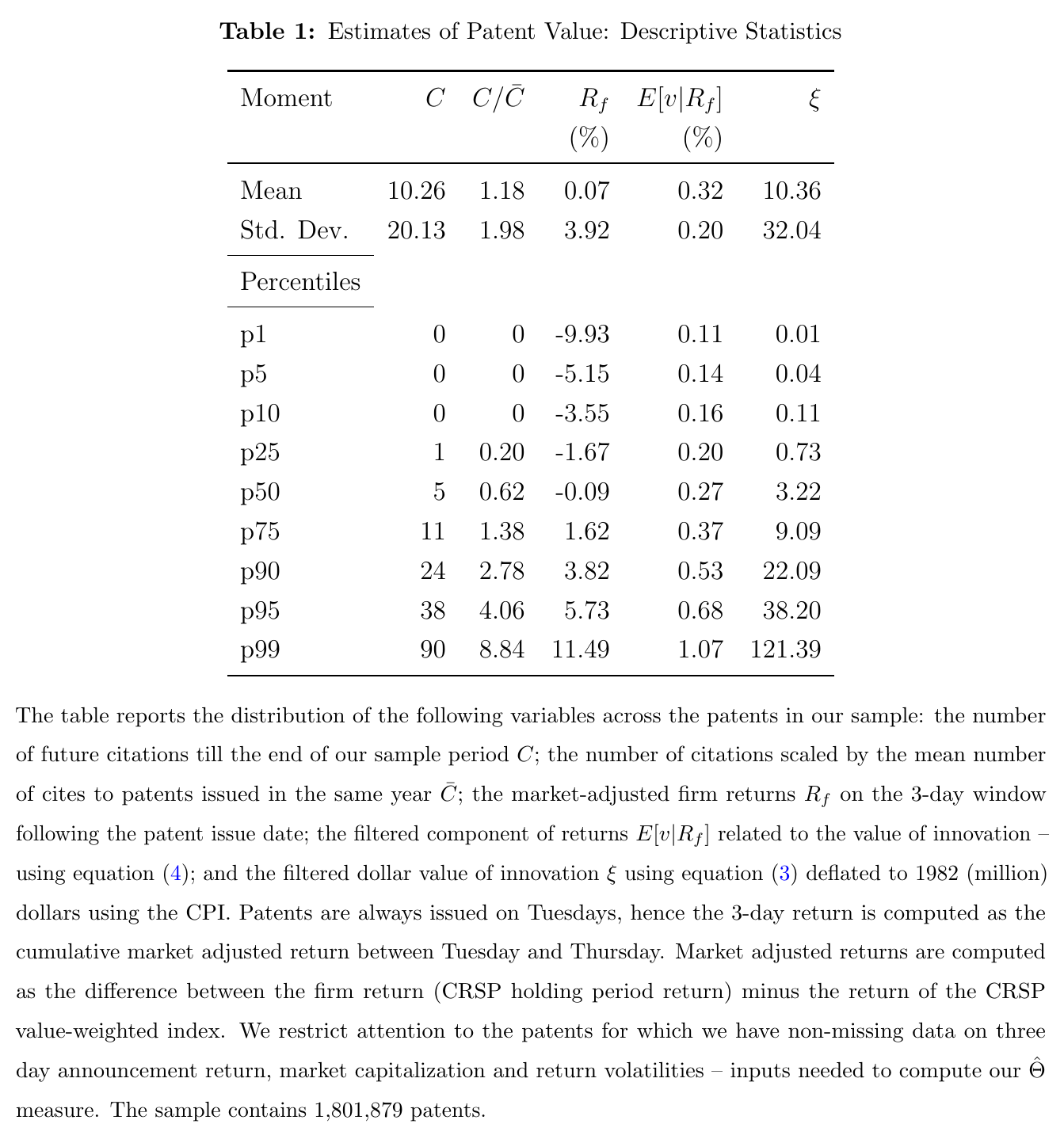
Table 1 gives the distribution. In 1982 dollars, the median patent is worth $3.22 million, the mean $10.36 million, the 90th percentile $22.09 million and the 99th $121.39 million: a fat right tail, as you would hope. The filtered patent share $E[v|R]$ has a median of 0.27 percent of market cap, and its first percentile is still 0.11 percent. The authors concede that the levels look high next to survey evidence (Giuri and coauthors (2007) find about two-thirds of European patents worth under €1 million), list the reasons, and fall back on the position that cross-sectional differences “can still be meaningful.” That is the right position, and the rest of the paper mostly uses the measure in standardised form anyway.

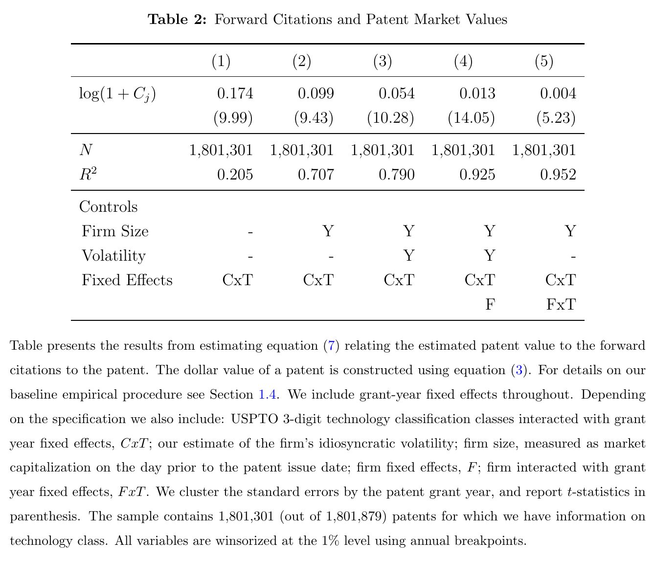
Is it measuring anything? Two checks. First, value and citations are positively related: in Table 2 the elasticity of $\xi_j$ with respect to $1+C_j$ is 0.174 with technology-class-by-year effects, and it stays positive and significant all the way down to 0.004 with firm-by-year fixed effects. Second, a placebo: re-run the whole exercise on 500 sets of fake grant dates drawn within the year, and the value–citation relationship disappears, which says the grant window carries information that a random window does not. Both checks show that the measure contains event-specific information. Neither validates the dollar level of any particular patent.

The evidence: innovators grow, and their rivals shrink

The firm-level object is the sum of a firm’s patent values in a year, scaled by its book assets, $\theta_{f,t}$, and the same thing for every other firm in its three-digit sic industry, $\theta_{I\setminus f,t}$. Then the growth regression:

This is eq. 12 in the paper: $X$ is profits, output, the capital stock, employment or revenue productivity (tfpr), $\tau$ runs from one to five years, $a_\tau$ is the loading on the firm’s own innovation, $b_\tau$ the loading on its industry rivals’ innovation, and $Z$ collects the lagged dependent variable, size, idiosyncratic volatility and industry and year effects.

The theory the paper appeals to is generic Schumpeterian growth in the Aghion–Howitt (1992) mould: a firm that innovates gains, and a rival’s innovation hurts it, “directly through business stealing or indirectly through changes in factor prices.” The sample is 158,739 firm-years for 15,787 public firms over 1950–2010, with financials and utilities dropped, and both innovation variables measured in standard-deviation units.

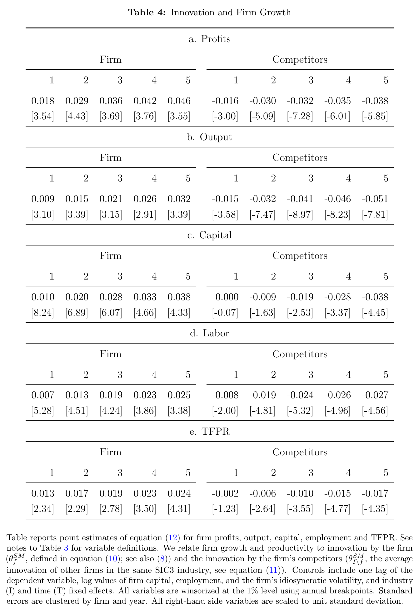
Table 4 is the headline. Over five years, a one-standard-deviation increase in the firm’s own innovation is associated with growth that is 4.6 percent higher in profits, 3.2 percent in output, 3.8 percent in the capital stock, 2.5 percent in employment and 2.4 percent in tfpr. A one-standard-deviation increase in rivals’ innovation goes with growth that is 3.8 percent lower in profits, 5.1 percent in output, 3.8 percent in capital, 2.7 percent in employment and 1.7 percent in tfpr, all with large t-statistics. The rival effects build with the horizon: for the capital stock the one-year coefficient is zero and the five-year one is $-0.038$. That is creative destruction showing up as a firm-level correlation.

Two terminological notes before anyone runs with these numbers. The text calls one outcome “capital investment,” but the variable is growth of the deflated capital stock, not an investment flow. And the text calls output “nominal,” but the table note deflates sales plus inventory changes by the cpi. Neither is physical output or physical productivity: tfpr is revenue productivity, and the authors themselves note that a rival’s innovation can lower it through prices and markups without anybody’s machines getting worse. And the paper is explicit that the relation “is based on correlations and cannot be interpreted causally.” Fast-growing firms may simply patent more.

The one surprising thing: the same patents, weighted by citations, show no creative destruction

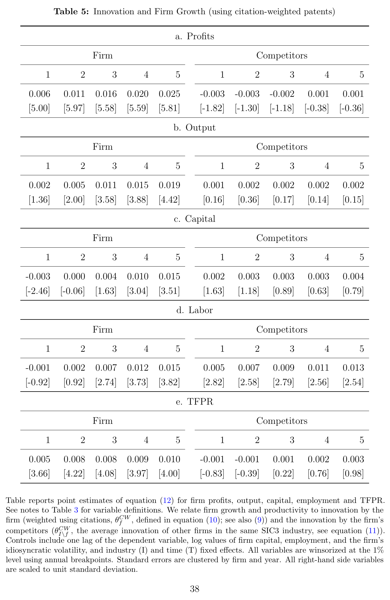
Now rerun eq. 12 with the conventional measure: each patent counts as one plus its citations relative to its cohort mean, summed by firm-year and scaled by assets (eq. 9). The own-innovation effects shrink: at five years they are 2.5 percent for profits, 1.9 for output, 1.5 for capital, 1.5 for employment and 1.0 for tfpr. The paper says “typically less than half” of the market-value ones. Against Table 4 the ratios run from about 39 to 60 percent, so call it roughly half. The interesting part is the rival column. Rivals’ citation-weighted innovation has insignificant or positive coefficients, and for employment it is significantly positive at five years. The same patents, weighted two ways, give opposite answers to the question of whether your competitors’ inventions hurt you.

When both measures go into the same regression, the market-value coefficients barely move, rival effects included, while the citation-weighted own effects weaken and its rival effects stay positive. The authors’ reading is that citations track scientific value, which spills over to neighbours, while market values track private value, which is partly taken from neighbours. That is a reasonable reading, and it is the cleanest way to see what the stock market adds. A citation is an acknowledgement, and acknowledging someone’s idea is often how you build a competing product on it. A stock-price jump is a forecast of rents, and rents in a product market are partly a transfer. The measure that sees business stealing is the one built from the beneficiary’s own valuation. (It doesn’t follow that the citation measure sees only spillovers and the market measure only stealing: both are mixtures, and neither regression separates them.)

In the online appendix, scaling by market cap shrinks own effects by about a third and enlarges rival effects; R&D and investor-attention controls leave signs and significance in place; and an instrument built from state R&D tax prices, following Bloom, Schankerman and Van Reenen (2013), gives the same signs with much larger coefficients and only marginal own-firm significance, which the authors fairly generously call “qualitatively similar.”

The paper also aggregates the firm coefficients into an accounting exercise: innovation, so measured, accounts for 5–23 percent of realised net growth among surviving public firms and 6–19 percent of the dispersion across them. With citation weights, the creative-destruction part of that accounting is “essentially zero,” which is the sign flip again in aggregate form. This is accounting with fitted values from correlations, and year fixed effects absorb anything general-equilibrium, so it is not a causal decomposition.

The aggregate index: new-patent value over output as growth news

The last step sums every patent’s value in a year and divides by output:

This is eq. 18 in the paper: $\Theta^{sm}_{ft}$ is the summed dollar value of firm $f$’s patents granted in year $t$, $F_t$ the set of sample firms, and $Y_t$ aggregate output.

Why divide by output? In the paper’s Appendix A there is a variety model in the style of Atkeson and Burstein (2011), where a competitive final-goods sector aggregates patented intermediate goods with a ces elasticity, each owned by a monopolist, and quality-weighted variety grows at an i.i.d. rate $\chi_t$. Value each patent with the household’s stochastic discount factor and the value of the year’s new patents over output comes out proportional to $\chi_t/(1+\chi_t)$, which is approximately the growth of the technology frontier. So the index is, to first order, frontier growth priced by investors. In the model the stock market is a constant multiple of output, so dividing by aggregate market capitalisation should give the same index. That second version is the paper’s answer to the worry that the index just tracks discount rates or bubbles: if the numerator rises because all stocks are expensive, the denominator should rise with it. The two indices correlate 0.89 in levels and 0.75 in first differences.

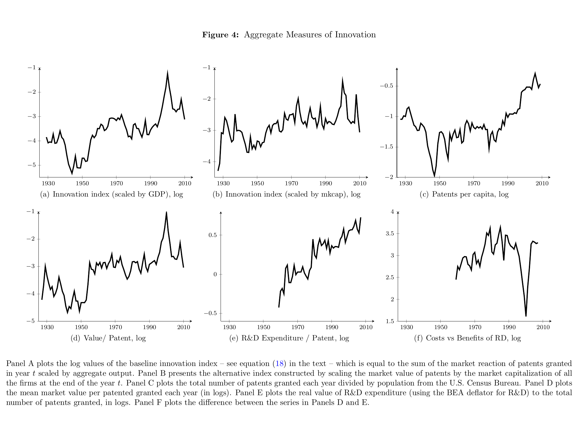
Figure 4 is the picture worth looking at. The index has three humps: the 1930s (General Motors, at&t), the 1960s and early 1970s (ibm, ge, 3M, Exxon, Kodak, du Pont, Xerox) and the 1990s–2000s (Sun, Oracle, emc, Dell, Intel, Cisco, Microsoft, Apple). (The introduction lists “the 1920s” for the first wave; the body and the figure say the 1930s.) Most of its low-frequency movement comes from value per patent, not from the number of patents, and the post-1980 explosion in patent counts that partly reflects legal changes barely registers. The correlation of the index with log patent counts is 60–75 percent in levels and only 14–18 percent in differences. The same decomposition gives a side result on Kortum’s (1993) puzzle of rising R&D per patent: R&D per patent rises secularly, but net of rising value per patent the cost-benefit ratio shows what the paper calls “a markedly slower decline.”

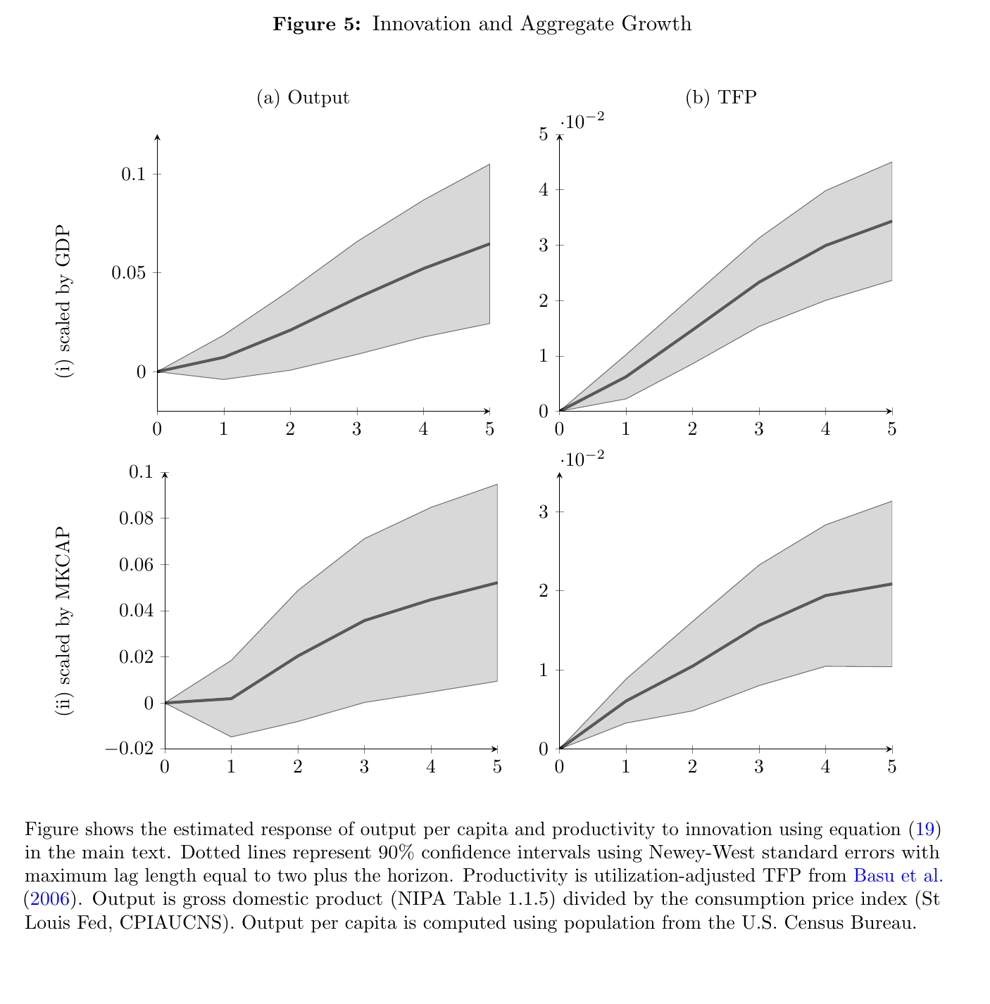
Then the growth regressions (eq. 19): the change in log output per capita, or in utilisation-adjusted tfp from Basu, Fernald and Kimball (2006), from $t$ to $t+\tau$, on $\log\hat\chi_t$ plus lags of the dependent variable, with Newey–West errors. Over five years, a one-standard-deviation higher index is followed by output that is about 6.5 percent higher and tfp that is about 3.4 percent higher. With the market-cap-scaled index the tfp response is 2.1 percent, and the output response is 5.5 percent in the text, though the figure’s panel ends closer to 5.2. These are cumulative level differences over five years, not annual rates, and the paper’s verb is “followed by,” which is the right one.

For a reader coming from growth and asset pricing, this is where the paper earns its place. The usual problem in that literature is that the slow-moving component of expected growth is very hard to see, and you end up inferring it from prices that are supposed to be responding to it. Here the price is the instrument on purpose. Investors’ valuation of the year’s new patents, divided by output, is a candidate observable for news about medium-run productivity, and it does predict output and tfp one to five years out. At the firm level the same instrument records displacement: the arrival of a rival’s valuable patent is associated with lower profits and output for incumbents over the following five years. In the paper’s own model (my reading, not the authors’), an old patent’s value moves with $Y_t/X_t$, which falls as the frontier grows once the ces elasticity exceeds two, so the displacement of incumbents’ assets is already there in the algebra. But the paper itself estimates no risk premium, no innovation factor and no long-run-risk process, and its model’s frontier growth is i.i.d. Turning displacement into a priced risk is the job of later work, including Kogan, Papanikolaou and Stoffman (2020), along with Gârleanu, Kogan and Panageas (2012) on displacement risk and Kung and Schmid (2015) on R&D as a source of long-run risk. This paper supplies the measuring stick.

Weak points, my own reading (no discussant exists)

The filter gives every patent a positive value that owes more to the firm than to the return. At a zero return $E[v|R]$ is about a tenth of the firm’s noise volatility, and 99 percent of patents get more than a tenth of a percent of market cap, so a patent’s dollar value is largely market cap times a volatility-dependent constant, plus a modest term that depends on the return. Cross-patent variation in $\xi$ is therefore driven heavily by firm size and volatility, which is exactly why the Table 2 elasticity falls from 0.174 to 0.004 once size and firm-by-year effects come in. “Strongly related to citations” leans on comparisons across firms.

Holding $\delta$ fixed across firms, industries and 85 years is a strong restriction. The test the paper runs on it, comparing patents filed in the months either side of the 2000 change that made applications public, compares one month to one month, and a null there says little about whether the timing of information is constant. Grant-day news may also be about more than the patent: the pipeline behind it, its enforceability, the odds of the next grant.

Most firm-years have no patents at all, and the rival variable is an aggregate across a three-digit industry, weighted by market value. An industry-wide valuation boom, of the kind visible around 2000 in Figure 4, would load on rivals’ measured innovation and could precede mean-reverting outcomes for everyone in the industry. Market-cap scaling does not dispose of this, since the rival effects get larger rather than smaller under it. Three-digit industries need not be the real competitors, private entrants are missing, and the instrument’s exclusion restriction needs tax prices to work only through patented innovation.

The aggregate evidence is about eighty annual observations with overlapping five-year changes. The 6.5 percent output response has a 90 percent band of very roughly 2.5 to 10.5 percent read off Figure 5. The bivariate var versions in the online appendix are smaller, with output bands that include zero (the tfp bands do exclude it), and the footnote describing them does not quite match the figure. A forward-looking price can predict output through expected demand or financing conditions as well as through technology, so “followed by” really is the claim. The appendix model is a measurement device rather than a test: the proportionality result needs i.i.d. frontier growth, all goods patented and markups fixed by the elasticity, and it contains no business stealing between named firms, so the firm-level creative destruction is not derived from it. There are a few slips in the documents too: a table in which one panel’s rival t-statistics duplicate the previous panel’s, Newey–West lag lengths that differ between text and figure note, and a footnote that calls a figure a table.

None of which takes away from what the paper did. Before it, the standard answer to “how much was that invention worth?” was a count of how often other inventors mentioned it. After it, the answer is what investors paid for it the week it was granted. That turns out to be a different number with a different sign for the neighbours, and the neighbours’ sign is the interesting one.

References