A Model of Global Firms and Capital Markets

Loukas Karabarbounis, Bruno Pellegrino and Juliana Salomao, “A Model of Global Firms and Capital Markets,” presented by Karabarbounis at the nber International Finance and Macroeconomics Program Meeting, 23 October 2026; discussant Ṣebnem Kalemli-Özcan. Version used: nber Working Paper 35652, August 2026, alongside the authors’ slides. The recording has no audio for roughly the first fifteen minutes of the talk, so the opening of the model rests on the paper and the slides, not on anything said in the room.

You run a listed firm in Brazil. Foreigners do not buy much of your stock, because something shaves their return on it, and the model is relaxed about what. So you raise less equity, which means you have less capital, make less output and sit further up your demand curve at a higher price. An American who would have bought your product now pays more for it, or buys something a bit worse. Nobody at any customs house collected anything. What you have is a tariff, levied at the stock exchange and paid at the checkout.

That is the idea in this paper: a capital-market friction is a goods-market friction with a longer route. Anyway, here is Karabarbounis on why that makes the two kinds of liberalization partly the same thing:

Look, the consumer doesn’t care, in the end the consumer cares about the utility from consuming these global firms. And both tariffs and financial frictions are gonna basically raise the price of inputs.

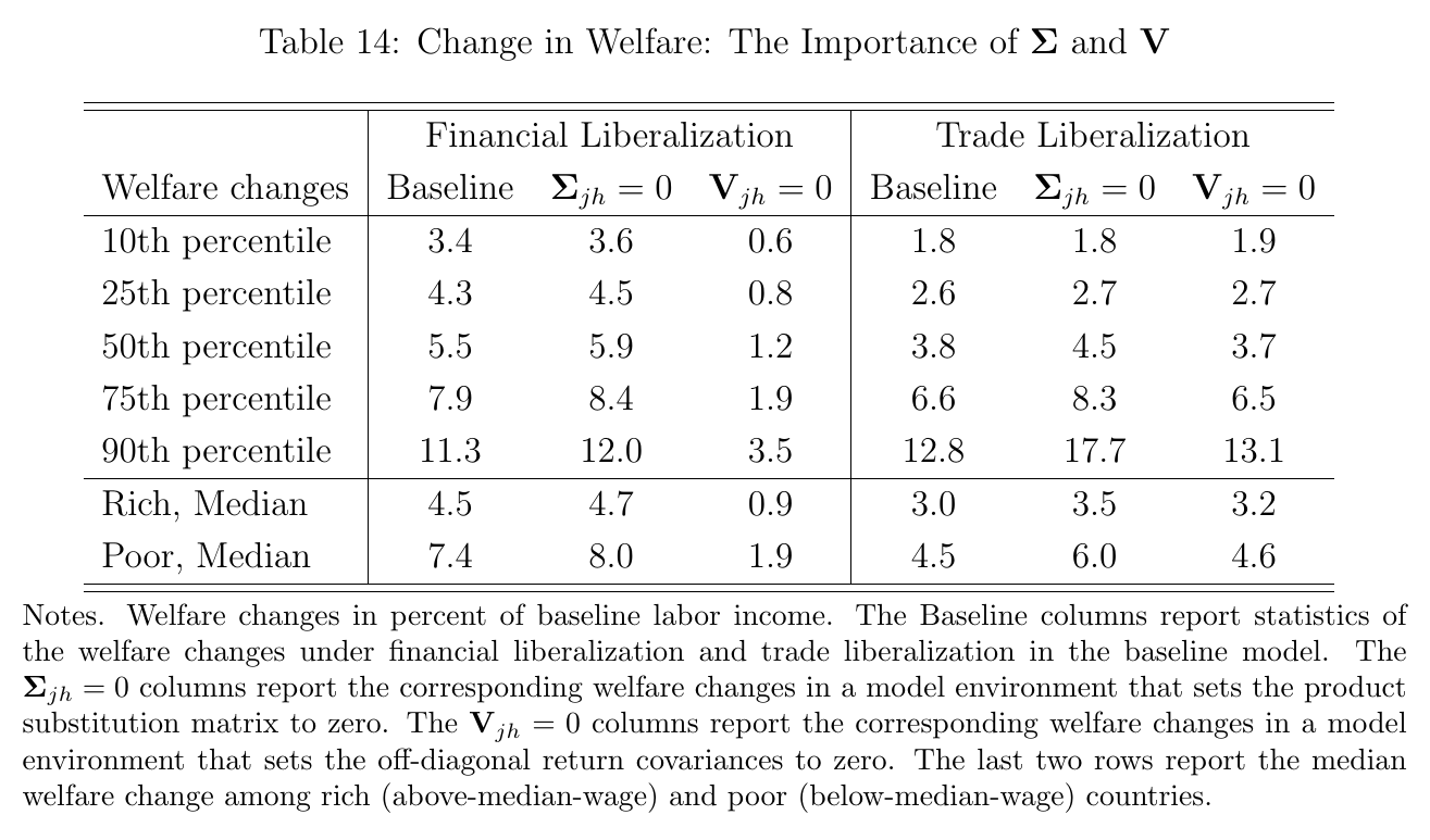
The authors build this for about 23,000 listed firms in 48 countries, each with its own product position, revenue footprint, labor footprint and shareholder base, and fit it exactly. Then they delete frictions. Removing every international financial wedge raises welfare in the median country by 5.5 percent of labor income. Removing tariffs and non-tariff measures, and leaving shipping costs alone, raises it by 3.8 percent. You might expect the first number to be diversification, and it is not. The term for portfolio variance is small, and in the emerging markets the gain is nearly all consumer surplus, which is to say cheaper stuff. (In rich countries like Japan, France and Germany the returns term does more of the work. Karabarbounis’s “the entire gains come from the consumer surplus” is true of the cross-country mean, and the paper’s version is more careful.)

The model: one loop through two markets

Investors in each country split wealth between a safe technology paying $r_0$ and the world’s equities, by mean-variance rules. A firm’s equity becomes physical capital at a fixed firm-specific rate $\chi_j$, which Karabarbounis calls reduced form: “we take it as given.” Capital becomes output one for one, and labor is hired wherever the firm happens to be: “Apple hires Indians from India and they pay the Indian wage.” More output pushes the firm’s price down a linear demand curve, and pushes down the prices of firms selling similar things. Lower price means lower profit per unit of capital, so a lower expected equity return $\mu_j$, so less equity. Equilibrium is where this loop closes, and because both sides are linear it closes in closed form once wages are given: “The only thing you need to put on the computer is the labor market clearing condition.” Wages do get re-solved in every counterfactual, with non-traded firms and labor supply supplying the only curvature, so the closed form is a statement about the core and not a claim that wages stand still.

Two pieces of housekeeping matter later. Firms here are price-takers, and “markup” in this paper is a profit share, with the inverse elasticity set equal to it by assumption, so when the talk says firms “charge” something you should translate. And the whole thing is static, one cross-section, listed firms, portfolio equity. Market cap is capital, firm by firm.

The interesting object is what the paper calls the transmission matrix, built from two measured matrices. $\boldsymbol\Sigma$ is product similarity, from Pellegrino’s text analysis of business descriptions extended to the whole world: you read what Apple does and what Samsung does and take a cosine. $\mathbf V$ is the covariance of returns. A common good shock helps firm $j$ directly and hurts it through everyone else’s expansion, and the net sign depends on where you sit in those matrices. For big firms it is positive. For small firms it is negative, so a reform that directly helps a small firm can still shrink it: “these guys basically are gonna be squeezed out from the liberalization.” (The paper derives the sign for a common shock with elastic labor. An actual liberalization is only similar.) Implied demand elasticities run from about −5 or −6 for the smallest firms to about −2 for the largest, which is the other reason size wins.

How you measure a friction nobody observes

Tariffs you can look up. The financial wedge you have to infer, and the inference has one identifying assumption, which is that residents face no friction at home. Then take holdings as data and read the first-order condition backwards:

Here $\mathbf S$ is the matrix of portfolio shares by firm and investor country, $\mathrm{dom}(\cdot)$ picks each firm’s home-investor entry, $\gamma$ is risk aversion (set to 4), and $\boldsymbol\Delta$ collects the wedges $\delta_{ji}$, a negative one lowering country $i$’s return on firm $j$. In words: if residents hold a lot of a risky, badly hedging home stock, it must pay well, and if foreigners then decline that good return, something must be stopping them. Karabarbounis’s example is Russia. Russians hold Russian firms despite high variance and poor hedging, so the inferred return is high, and “no one else invests in Russia. So it has to be that they have high deltas.”

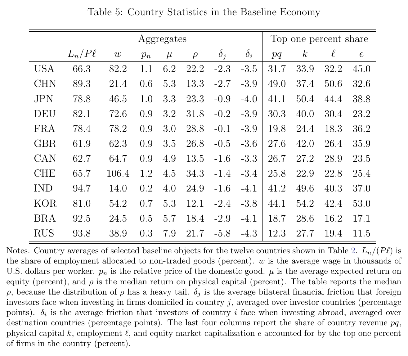
The model then matches firm by firm, so no moment is left over to test it. The inferred firm-level returns get a smell test instead. The highest among large us firms are Tesla and Nvidia, and Karabarbounis says they “kind of smell right to me” and allows that it could be done more formally. The paper is candid in a footnote that $\mu_j$ “need not coincide with realized average returns.” Note the asymmetry, which will matter: the trade friction is measured from outside the model and the financial friction is whatever the model needs.

The two experiments

Set $\boldsymbol\Delta = \mathbf 0$ with everything else fixed. Equity expands, since investors move out of the safe asset, and dispersion across firms jumps: the standard deviation of log equity changes rises 25 points and the 90–10 gap 57. Mean revenue falls, because production rises and prices fall. By country the median is 5.5 and the mean about 7, from about 3 in the us to about 10 in India. It is a far-out experiment. Every country ends up holding the same 36.2 percent in the safe asset, and foreign equity goes to 54 to 63 percent of wealth almost everywhere. The usa, at 36.1 percent foreign with 27.7 still at home, is the exception that keeps home bias from vanishing altogether. The paper’s framing is that the observed world is “closer to financial autarky” than to this.

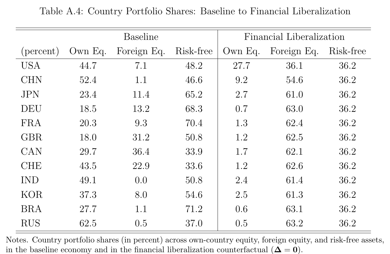
Trade liberalization removes tariffs and non-tariff measures and keeps shipping, which Karabarbounis treats as a technological constraint, and also keeps home bias in preferences. Now the world as a whole leaves its split between equity and the safe asset about where it was, though individual countries do shift, and the reallocation runs within equity. Revenues go up instead of down, because this is a demand shock and the financial one was a supply shock. Karabarbounis says the 3.8 is comparable to what trade economists get in a different experiment, and the model’s implied trade elasticity is about −4 (the paper has −4.29 in levels and −3.58 in changes).

Now run each experiment in a world without the other friction. If the frictions were separable, nothing would change. Instead, for the median below-median-wage country, the trade gain falls from 4.5 to 3.1 and the financial gain from 7.4 to 5.8. The authors’ conclusion is that the liberalizations are substitutes and the frictions amplify each other: removing one does part of the other’s job, and emerging markets gain more because they have a lot of both. For rich countries the difference is slight. The pitch to the two audiences follows, and it is a good one. If you do international finance you need trade frictions in your model, and if you do trade you need financial ones.

Three things to hold alongside that. The world without trade frictions here removes shipping as well, so it is not the policy experiment. No table in the paper runs both liberalizations together. And “substitutes” comes from a model with one channel between the markets, so nothing in it could point the other way.

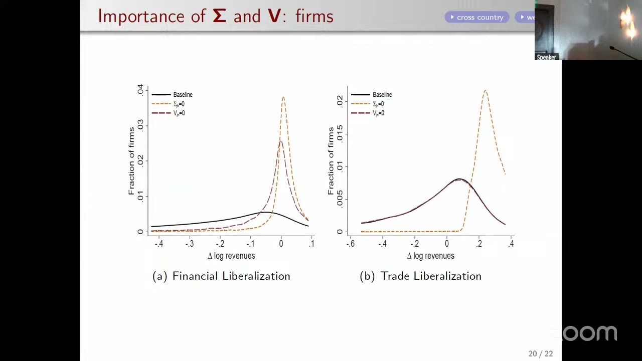
The matrices matter a lot for who loses. Shut off product substitution and, in the paper’s words, you eliminate “nearly all the negative equity and revenue changes under trade liberalization” and substantially reduce them under finance. Almost everybody wins, and the trade gains grow (the 90th percentile country goes from 12.8 to 17.7). Competition is what manufactures the losers, and it also holds down the winners.

The one surprising thing

Make stocks uncorrelated. Set the off-diagonal return covariances to zero and recalibrate. The textbook says the less your foreign stocks move with your home stocks, the more you gain from going abroad. In this paper the median financial gain falls from 5.5 to 1.2, so 78 percent of it goes away, while the trade gain barely notices (3.8 to 3.7). Kalemli-Özcan’s slide puts it as “less value from diversifying, bigger gains,” and the spoken version is that you have to “go through it a couple of times to wrap your head around” it.

The resolution is that this is an inference result. Look back at (31) and (32). $\mathbf V$ is in the measuring device. Positive covariance is what makes a home stock a bad hedge, so holding it implies a high $\mu$, and foreigners not holding a high-$\mu$ asset implies a large wedge. Zero out the covariances and the same portfolios imply lower returns and smaller wedges, so there is less to remove. The paper’s own sentence is that “without asset correlation, the inferred international financial frictions are much smaller and so the gains of removing them are smaller.” The experiment is not the same economy handed a better diversification opportunity. It is a different reading of the same holdings, and the gain is denominated in wedge, and the wedge is proportional to $\gamma\mathbf V$. (That account covers the welfare number, and the paper offers it. $\mathbf V$ also moves firm-level dispersion directly through the transmission matrix, and nothing in the paper separates the two channels.)

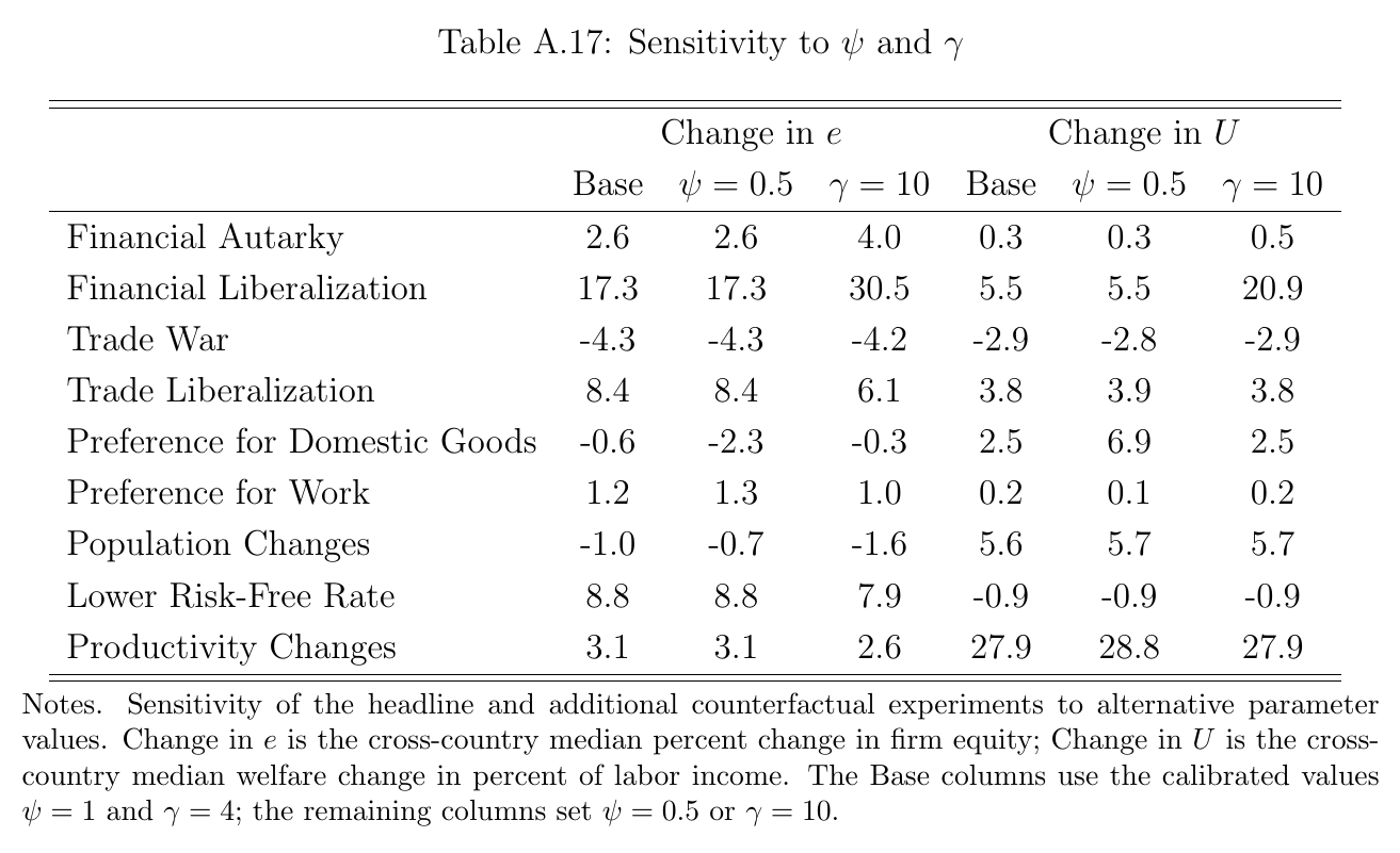
Two further things follow, and both are my reading. First, the experiment zeroes every off-diagonal pair, including pairs inside a country. Portfolios are mostly domestic, so the covariance doing the work in (31) is largely domestic covariance. Kalemli-Özcan’s framing, that Korean and us stocks moving independently would leave nothing to gain, is therefore not quite the experiment run, and zeroing only the cross-border pairs might do much less. Nobody has tried it. Second, $\gamma$ sits right next to $\mathbf V$ in the same two equations, and it is assumed. Table A.17 sets it to 10 and the median financial gain goes from 5.5 to 20.9, while the trade gain stays at 3.8. The paper says this “substantially increases” the gain and moves on. The trade friction is measured, so it does not care. The financial friction is a residual scaled by an assumed number, so it does, though the factor of 3.8 on a 2.5-fold rise in $\gamma$ is more than simple scaling would give, and the paper does not derive it.

What Kalemli-Özcan pushed on

The discussion began in real affection (“a new workhorse”) and then took the result apart in the right order. The recording has no reply from the authors to any of the points below.

Start with $\mathbf V$, which does the heavy lifting: a 23,000 by 23,000 matrix from daily returns in a single year, and that year is 2023, with Russia under sanctions, policy rates at their peak and the ai boom underway. Holdings and returns also come from different years, and non-synchronous trading pushes covariances down. The suggestion is a factor model on weekly returns over five years, with some thought about currency. (Before the discussion Karabarbounis had said that going back in time runs into missing data for many variables.)

Then $\boldsymbol\Delta$. The levels are not crazy, as Kalemli-Özcan agrees, but “it is still a residual and it absorbs everything”: capital controls, currency risk, hedging labor income, information, institutions. Trade reform in this paper removes the measured policy part. Finance reform removes the whole residual, including things no finance minister can repeal. So project $\boldsymbol\Delta$ on capital controls, taxes and distance, and liberalize the policy part only, as is already done on the trade side. There is also a us puzzle: a bigger wedge on the us than on India, while the us share of global portfolios surged after 2017. Part of that puzzle is built in at the data step, since the bilateral shares are 2017 shares scaled by 2023 aggregates, so a post-2017 surge cannot reach them at all. The other half is the high inferred us return, which comes from the 2023 $\mathbf V$ and the 2017 shares, and whether vintage moves it is untested.

The sharpest point is the home assumption. “You cannot do this identification with frictions at home,” and residents plainly face them. Kalemli-Özcan says the inferred returns of 7.9 for Russia and 5.7 for Brazil are too high, so foreign wedges and gains are too large, and the slide says these frictions hit residents and foreigners alike. The algebra here is worth a moment, and it is mine, from the first-order condition behind (31) and (32). With a true home wedge, the paper recovers $\mu_j$ plus that wedge and a foreign wedge net of it, so only foreign-minus-home is identified. A friction hitting residents and foreigners equally cancels out of $\boldsymbol\Delta$, and is neither inferred nor removed. So “$\boldsymbol\Delta=\mathbf 0$ deletes bad institutions” holds only for the part that discriminates against foreigners. And “$\mu$ too high” needs a positive home wedge, meaning captive domestic savers holding more than the return justifies. That fits financial repression, and it does not fit weak minority protection, which residents bear too and which pushes the inferred return the other way. The point survives, with a narrower object than the slide’s wording. The proposed fix, dual-listed firms, seems like the right kind of data.

Then China. “If China opens tomorrow, the model is going to say money is going to pour into Chinese stocks,” whereas Kalemli-Özcan’s guess is that Chinese savings pour out, and this is “first order.” The model does have that outflow: Chinese foreign equity goes from 1.1 to 54.6 percent of wealth, about $11 trillion, and own equity from 52.4 to 9.2. But foreigners pile in by more. On my arithmetic from the paper’s rounded portfolio tables, net foreign ownership of Chinese equity goes from about $1.6 trillion to about $4.5 trillion (at least $2 trillion on the stingiest reading). So Kalemli-Özcan reads the model correctly, in net as well as gross, and the disagreement is with its prediction. Two caveats on the prediction: the paper’s experiment opens every country at once, not China alone, and it compares stocks with no transition, so “pours in” means a change in who owns Chinese firms.

Three shorter ones. Equity equals capital in the model, whereas in data valuation moves first and investment lags, with liberalization episodes as a benchmark to test against (the slide cites Henry: 38 percent revaluation on announcement, growth up a point a year). Debt and fdi, not listed equity, are most of what reaches emerging markets, so the results are “equity liberalization for listed firms.” Substitutes is one channel, and there is a whole literature of complementarity stories (Antràs and Caballero (2009), Obstfeld) the model cannot express. FactSet allocates unreported regional revenue in proportion to gdp, which the paper confirms, and that may overstate foreign sales into India, where the foreign spending share is 53 percent. And with no friction inside countries, concentration among large firms is efficient by construction. Kalemli-Özcan points to Spain and Hungary going opposite ways on misallocation and would like a wedge on the marginal product of capital in the model.

The room

Most of the Q&A survives only in part: the opening is lost, and much of the answering is garbled. One questioner said they least believe welfare numbers about big reforms, and that the framework’s advantage is smaller questions, like whether the Washington consensus suits a country with “very uncompetitive” firms and whether India should have liberalized trade before the capital account. The answer is mostly gone, and no sequencing calculation exists. Another asked what the characteristics demand system actually delivers for trade economists, number or mechanism. Karabarbounis: “the number is the same, but the mechanism is different.” A co-author added that opening the capital account lowers the required return, so firms “endogenously charge lower markups” at home and abroad, which is “absolutely unique to our model.” (Spoken claim. The paper’s introduction cites other work with risk in markups, and these firms take prices as given.) A third raised vertical integration and the skill bias of the Revelio data. The audible answer is that the non-traded sector exists to keep the allocation of labor from being off, which helps with sector sizes and leaves a firm’s geographic footprint where it was. There is no audible answer on vertical integration.

Kalemli-Özcan closed by saying that the paper finds the world close to financial autarky at the border, that the frictions inside the border matter a lot, and that the framework is the thing to separate them with. That seems right, and the paper’s nicest property is that it says plainly what it is measuring. The textbook tells you to go abroad because foreign stocks do not move with yours. This model tells you to go abroad because they do, and if you would like a bigger answer, there is a risk aversion coefficient you could raise.

References