The Housing Boom and Bust: Model Meets Evidence

Greg Kaplan, Kurt Mitman and Giovanni L. Violante — Journal of Political Economy 128(9), September 2020, pp. 3285–3345; earlier as NBER Working Paper 23694. Written from the published article and its online appendix. There was no talk and no discussant.

It is 2003 and you are renting a house. It is the house you want; it has the number of bedrooms you want; you are renting it because you cannot come up with a down payment on a house that size, and buying a smaller one strikes you as a bad trade. Then credit gets cheap. The maximum loan-to-value ratio your lender will write goes above 100, the fee for originating the mortgage falls by nearly half, and a payment-to-income limit that used to cap you at a quarter of your income doubles. So you buy.

What do you buy? You buy the house you were already living in, or one very much like it. You wanted that much house before; you want that much house now. What changed is the financing, not the appetite. So the homeownership rate goes up by one household, and the aggregate demand for housing services goes up by roughly nothing, and the price of housing therefore does roughly nothing.

That is the paper. Kaplan, Mitman and Violante build a large equilibrium model of the US household sector, hit it with the three shocks everyone argues about — income, credit, and beliefs about future housing demand — and find that the credit relaxation of the 2000s has, in their words, “a trivial impact on house prices” (p. 3316), while doing most of the work on homeownership, mortgage debt and foreclosures. Prices are moved almost entirely by beliefs. The authors nominate this themselves as the surprise: house prices are “almost completely decoupled from credit conditions” (p. 3289), and note the almost, because they mean attenuated, not absent.

The machine

Households live from 21 to 81, work until 65, get hit by uninsurable earnings shocks, and consume nondurables and housing services (p. 3302). Housing services come two ways. You can rent, which is frictionless — adjust every period, no transaction cost, no borrowing — or you can own, which yields a small extra utility flow, costs 7% of the house to sell, and requires clearing a loan-to-value limit and a payment-to-income limit at origination. Four supply blocks close the thing: financial intermediaries who price every mortgage individually at zero expected profit, a rental company that sets rent off a user cost, a construction sector with a land constraint that delivers a supply elasticity of 1.5 (the median metro area in Saiz, p. 3305), and a final-good sector linear in labour so the wage is just productivity.

Two features of that description are load-bearing and both are unglamorous. The first is that the rental option is a real, well-calibrated option rather than a corner. The extra utility from owning is worth about half a percentage point of consumption to the median owner (p. 3304) — a genuinely tiny number, and the reason the tenure margin is a hinge rather than a wall. The second is that mortgages are long-term, amortising, defaultable and refinanceable, so the two origination constraints bind at origination and never again. However far underwater you go, nobody can force you to delever as long as you make the payment (pp. 3295, 3320). Delete the rental market and everyone must own, so a large mass of households really is rationed in housing services and cheap credit really does raise prices. Delete the long-term contract and every price fall forces every owner to cut consumption to roll the debt, so housing becomes a terrifying asset with a large, credit-sensitive risk premium. Keep both, as the United States does, and the paper’s verbs are the right ones: the rental option “limits” the increase in housing demand, and long-term debt “reduces the strength” of the risk-premium channel (pp. 3289–3290).

Two equations carry the rest. The rental company’s user cost, equation (11) at p. 3299,

says the rent $\rho$ on a unit of housing is the operating cost $\psi$ plus today’s price $p_h$ minus the discounted expected resale value, net of depreciation $\delta_h$ and property tax $\tau_h$, with $\mathfrak{m}$ the discount factor and $\Omega$ the aggregate state. And the mortgage pricing function, equation (10) at p. 3298,

gives the price per unit of face value on a loan of size $m'$ to a household of age $j$ holding portfolio $\mathbf{x}'$, where $g^n$, $g^f$ and $g^d$ are the indicators for selling, refinancing and defaulting, $\zeta_m$ is the origination wedge, $\kappa_h$ the sale cost, $\delta^d_h$ the extra depreciation on a foreclosed house, and $\pi$ the mortgage payment.

The dials, and the shock that isn’t one

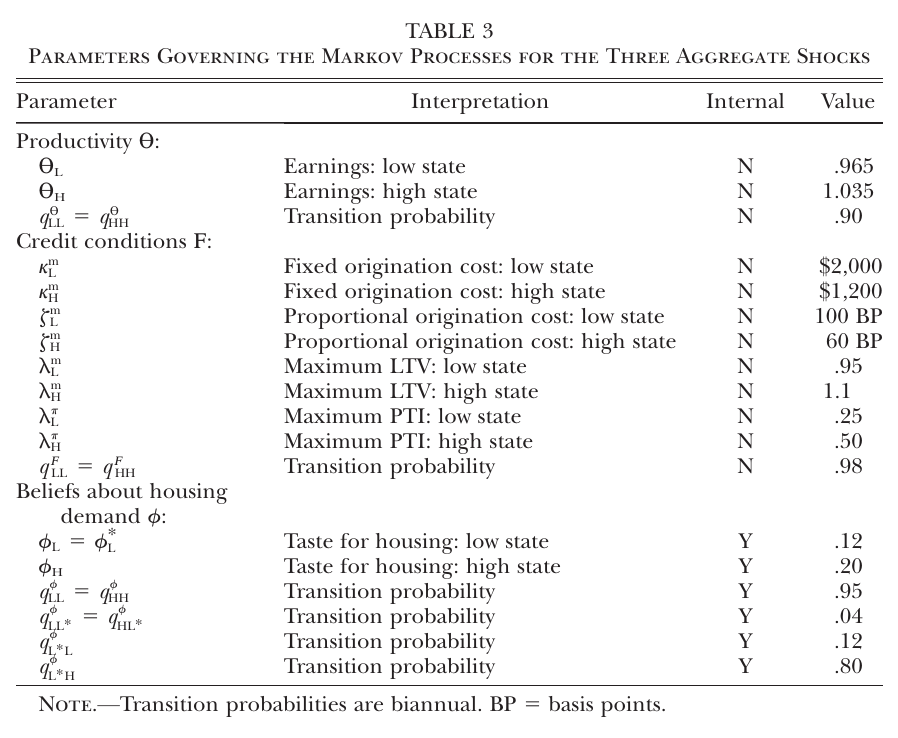
Productivity and credit are what you would expect: the wage swings, and an index bundling the LTV limit, the PTI limit, the fixed origination fee and a proportional wedge moves between two states. The belief shock is the clever one, and it is worth slowing down. There are three belief states but only two distinct values of the taste-for-housing parameter $\phi$. The low state $\phi_L$ and the starred state $\phi^*_L$ carry the same preference parameter. They differ only in where they are likely to go next: from the starred state, an 80% chance of the high-taste state next period; from the plain low state, one percent. So switching from $\phi_L$ to $\phi^*_L$ changes nothing whatsoever about what anyone wants today and everything about what they expect to want tomorrow. It is, as the authors put it, a news shock about a fundamental parameter that “shares the key features of a rational bubble” (p. 3286). In the boom-bust experiment the economy runs $\phi_L \to \phi^*_L \to \phi_L$: the preference change never actually happens. Everyone simply believes for six years that it might.

The boom itself arrives in pieces. The body text compresses it into a combined switch in 2001 reversing in 2007 (p. 3310), but the online appendix’s simulation description makes the sequencing explicit: productivity turns first, credit one two-year model period later, the belief switch the period after that, and all three revert together. The fundamentals move first and the optimism arrives last, which is roughly the order a narrative historian would have guessed. The ex ante probability in 1997 of drawing exactly this history is about 0.05% (p. 3311). The authors call it a tail event and do not squirm: agents always use correct conditional distributions; they just got an extraordinarily unlucky draw.

What each shock actually does

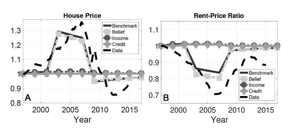
The benchmark gives a 30% rise in house prices and a similar-sized fall, and the belief-only line is nearly indistinguishable from it (p. 3316). The model also produces more than half the observed fall in the rent-price ratio, again almost entirely from beliefs, and equation (11) is why. The authors’ own gloss is the careful one: when current prices rise, rents rise too, and absent any change in beliefs the ratio “would remain roughly stable (or even go up, if the house price dynamics were mean reverting)” (p. 3317). It takes an increase in expected future prices — a bigger number subtracted on the right-hand side — to push rents down against prices.

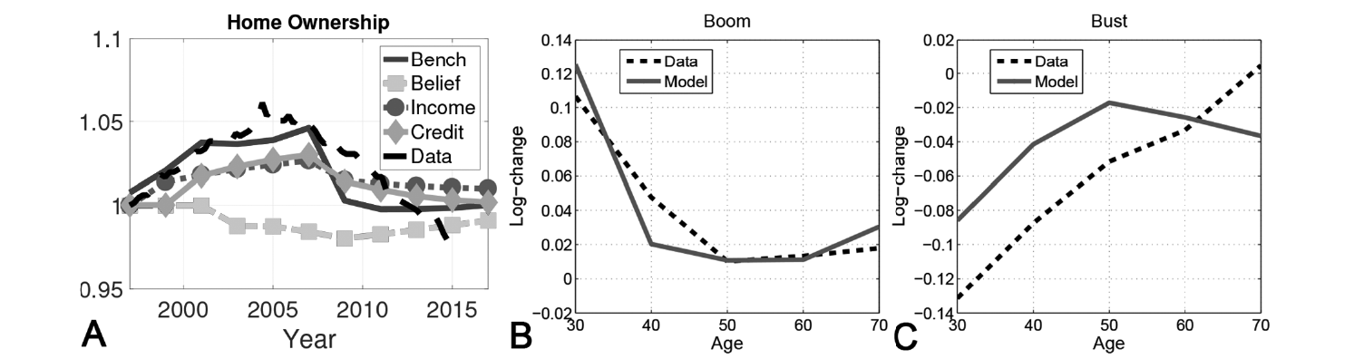
Now run it the other way. The belief shock on its own reduces homeownership during the boom, for two reasons the model hands you: the falling rent-price ratio makes renting comparatively cheap, and the higher price level makes the down payment bind for more households (p. 3317). Productivity accounts for a 3% rise in homeownership by relaxing the payment-to-income limit; the credit relaxation has a similar-sized effect through the LTV limit and origination costs. They do not sum to the benchmark, because of an interaction the authors state better than I can: “the belief shock makes more households want to own more housing, while the credit conditions shocks makes more households able to buy a house” (p. 3317). And in both model and data the swing is carried by the young, for whom both constraints actually bind — a fact of Hurst’s that the model reproduces without being asked to.

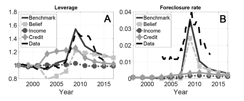
Leverage is where the argument locks. US leverage was flat through the boom, and the model gets it flat “because of two offsetting effects” (p. 3320): optimism raises prices and pushes the ratio down, looser credit expands debt and pushes it up. Neither shock delivers flatness alone. Beliefs alone drive leverage down to about 0.80; credit alone drives it up. The paper does not claim a formal identification result — the conclusion says only that the two findings together “epitomize how difficult it can be to separately identify the effects of credit supply shocks and shifts in expectations from micro data, without firm guidance from theory” (p. 3341) — but reading the decomposition, it is hard not to conclude that the two shocks are pinned down only by insisting on prices and quantities at the same time. That is my reading of the exercise rather than a sentence the authors write. It is also the paper’s cleanest weapon against the credit-only literature, and I will come back to it.

The foreclosure spike, meanwhile, is driven by the price collapse from the belief reversal, not by the credit tightening. The tightening “does not generate a spike” for two reasons the authors give: it does not move prices, and with long-term debt a tightening of the origination constraints is irrelevant to anyone who already originated (pp. 3320–3321). But credit relaxation amplifies the spike enormously, because it let optimists take out larger and cheaper mortgages at the peak, and then the price fall dragged them under. During the bust, mortgage debt stays well above its preboom level for over a decade: households delever by sticking to their amortisation schedules rather than by wrenching consumption cuts. Only those near their home equity line limit are forced to move quickly, and at the peak only about 4% of homeowners had used more than three-quarters of that line (p. 3320, n. 22).

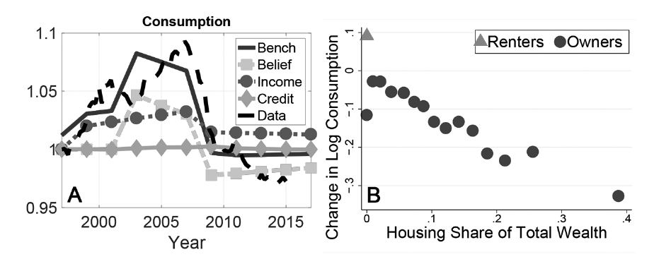
Consumption follows mechanically from all this. The credit shock has virtually no effect on nondurables because it has virtually none on prices; roughly half the consumption swing is labour income and the rest is the belief shock working entirely through house prices (p. 3322). The channel is a wealth effect, not collateral and not substitution: the consumption drop over 2007–11 is proportional to the household’s initial share of housing in total wealth, human wealth included, with a semielasticity “not far from one”. The genuinely subtle bit is why the aggregate wealth effect is nonzero at all, since a price fall is a gain for a renter saving a down payment and for an owner who plans to upsize by more than he owns. It turns on a life-cycle fact: both margins of housing demand have levelled off by age 40–45, so most households expect to climb down the ladder, and around 75% of households accounting for around 80% of aggregate consumption take a negative wealth effect (p. 3323). They have slightly smaller marginal propensities to consume than the other quarter; there are just far more of them. The aggregate elasticity of consumption to house prices comes out at 0.20, against 0.18 from applying the Berger et al. back-of-the-envelope rule to the belief-only version — a fully specified equilibrium model and a formula on a napkin landing in the same place, which is one way of establishing that the wealth effect really is the whole story.

Foreclosure as a savings vehicle

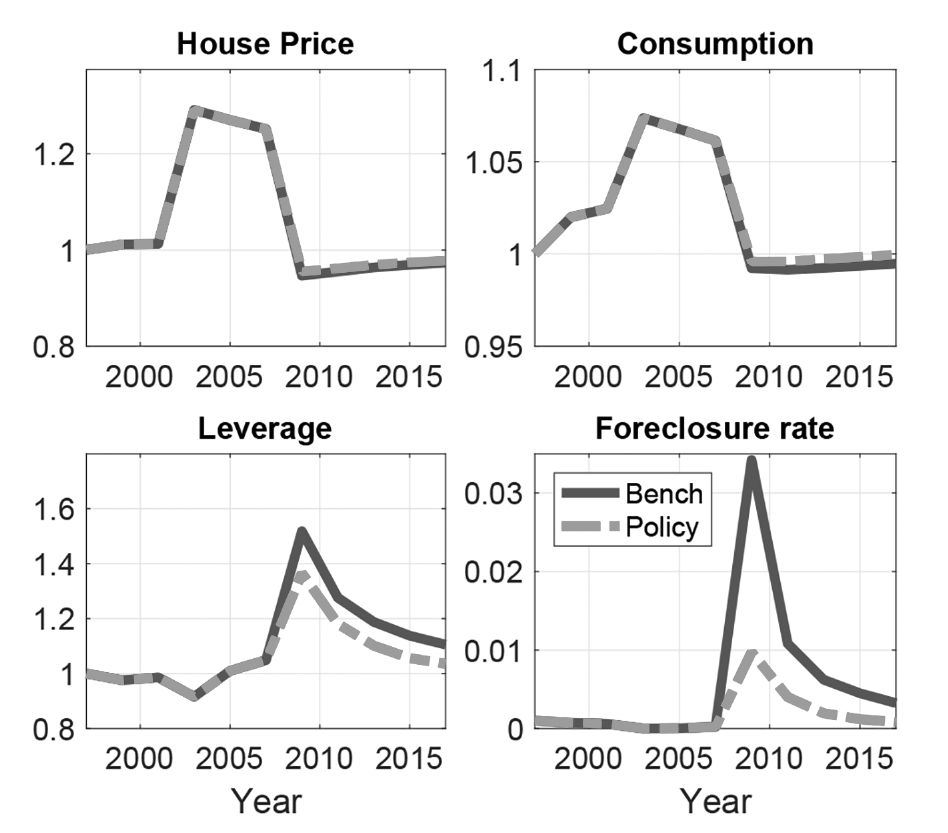
Here is the surprising thing. The paper runs the debt forgiveness program the 2009 critics wanted and nobody got: every homeowner above 95% LTV in 2009 has principal written down to exactly 95%, then repays on the baseline schedule. It reaches about a quarter of all mortgagors, far more generously than HAMP or HARP, and the government reimburses the lenders out of non-valued spending so there are no financing distortions (p. 3339). Foreclosures are cut by roughly three-quarters. House prices do not move at all. And the consumption decline through the bust does not move either — but not for the reason you would guess.

Because it is not just that credit is disconnected from prices, though it is. It is that foreclosure is itself a vehicle for consumption smoothing, so by preventing foreclosures the program makes the people it rescues consume less. Default, stripped of its moral packaging, is a lumpy transfer of resources from the lender to the borrower’s consumption: you stop paying, and the money you were paying becomes money you can spend. Households in the model who would have defaulted instead find themselves above water, keep making payments — “which they happily do to avoid the utility cost of default”, worth roughly 30% of a period’s consumption (pp. 3304, 3340) — and cut consumption to fund them. The program converts a group of people who were about to stop paying into a group of people who keep paying. This is good for them, good for their lenders, and very good for the foreclosure statistics. It is not good for their near-term spending.

One qualifier the paper insists on and I will not drop: the unchanged price path holds because the model has no foreclosure externality. The authors say so themselves — “Only large foreclosure externalities on house prices — not present in our model — might change this result” — and defend the omission by pointing to micro estimates of local spillovers that are small and highly localised (p. 3340, n. 40). The policy’s real payoff is real but oddly shaped: because forgiven principal means lower payments for the rest of the contract, and many of these households are near hand-to-mouth, consumption rises slowly as the payments arrive rather than all at once — about 0.3% a year for at least a decade (p. 3341). Agarwal and coauthors found exactly this in the HAMP data: no change in nondurable consumption, a real reduction in foreclosures. Ganong and Noel found that payment reduction moves spending while additional principal reduction does not. It is a good policy that works through none of the channels it was sold on.

A note on objections, and where the answers come from

There was no seminar here — no discussant, no Q&A. What follows are the objections the paper’s own Sections V.B through V.D and its online appendix are visibly built to pre-empt, with the paper’s own robustness results as the answers. Nobody asked these out loud; the authors asked them of themselves.

The first is that the credit relaxation has been modelled wrong — that the boom was about home equity extraction, or teaser rates, or the global savings glut. The appendix tries all three. Raising the home equity line limit from 0.2 to 0.3 does almost nothing, because the model matches the take-up distribution and only a minority of households were anywhere near their limit. Modelling adjustable-rate and teaser mortgages as a fall in the amortisation rate — a 7% average cut in minimum payments — also does almost nothing to prices or consumption. Dropping the risk-free rate from 3% to 2% does raise prices, with a semi-elasticity of about 5.5 against the 7–8 Glaeser, Gottlieb and Gyourko estimate, but the movements are far too small, it pushes homeownership and leverage the wrong way, and it has a structural problem the authors name up front: rates never went back up, so a rate story cannot generate the bust at all.

The second is that the whole no-price-effect result is an artefact of a frictionless corporate rental sector, when real landlords are leveraged households who ate the same credit shock. Section V.C answers this four times over, and one of the answers is unusually sporting: the paper generalises the user cost to include a landlord leverage wedge, a conversion wedge and a general discount factor, switches the belief shock off entirely, and then reverse-engineers time paths for those wedges so the model reproduces the observed rent-price ratio exactly — giving the credit story the same free hand the belief story got. All three wedges hit the rent-price ratio. All three fail on prices, because the adjustment runs through rents falling rather than prices rising, and all three then produce a counterfactual decline in homeownership (pp. 3334–3335). Cheaper credit for landlords makes renting more attractive; it does not raise the total demand for housing. A version with household-landlords who rent out spare units gives the same answer, and here the authors concede a real limitation instead of burying it: the annualised expected excess return on housing in their model is around 2%, or 3% with belief shocks, against the 5%–6% Giglio and coauthors estimate. “This is a limitation of our framework and poses a challenge for the literature” (p. 3336). That is the paper’s most honest sentence.

The third is Favilukis, Ludvigson and Van Nieuwerburgh, who get a large price response to the LTV limit in a model at least as serious. The answer is not that they are wrong but that the difference is fully diagnosable: no rental market, short-term non-defaultable mortgages, and higher risk aversion. Rebuild the Kaplan–Mitman–Violante model with those three features and credit relaxation alone generates a 20%–25% price boom-bust (p. 3338). Two things follow. First, “of the three features, the short-term nondefaultable debt and the absence of a rental market are the key ingredients” — it takes both deletions; raising risk aversion to 8 while keeping the rental market and long-term defaultable debt yields at most a 5% price swing against 35% in the data (p. 3338, n. 37). Second, and this is the knockout, the rebuilt model buys its price swing with a large counterfactual increase in leverage during the boom, and US leverage was flat. The price channel and the leverage channel are not independently adjustable. And the assumptions are simply wrong for the United States: a third of households rent, the median mortgagor in 2015 held a 30-year contract with only 2.6% holding contracts under 13 years, and roughly half the population lives in no-recourse states.

The fourth is the Mian–Sufi micro evidence, and it is the objection the paper converts most cleanly into support, because the consensus on those cross-sectional patterns has itself moved. Foote, Loewenstein and Willen find credit growth in the boom distributed uniformly across the income distribution rather than concentrated at the bottom; the model reproduces this, and reproduces it because of the belief shock, since everyone expects capital gains but high-income low-risk households are best placed to act on optimism. Albanesi and coauthors find the lowest-FICO quartile’s share of foreclosures fell during the bust; the model has no credit score, so it proxies one with each household’s equilibrium mortgage spread at origination, and reproduces the pattern for the same reason — prime borrowers who levered up expecting appreciation found themselves underwater.

Which leaves the two objections the paper answers by conceding. The 0.05% history really is a one-in-two-thousand draw, and that is the honest cost of insisting on a fully stochastic model with aggregate risk instead of a deterministic transition out of steady state, which is what most of the literature does. And the beliefs are exogenous: the boom is explained by an unexplained shock, and the conclusion says so, nominating learning from the low-rate environment as the most promising place to look next (pp. 3341–3342).

Anyway

The deepest thing in the paper is not the belief shock, which is a modelling device, however elegant. It is the demonstration that lenders’ optimism and households’ optimism land in completely different places. Strip the optimism from the lenders alone and leave everyone else believing, and prices, consumption and the rent-price ratio come out almost identical to the benchmark — but homeownership falls counterfactually, debt growth is a tenth lower (so lender beliefs account for nearly a third of boom-era debt growth), and the foreclosure peak collapses from 4% to 0.5% (p. 3327). Optimistic lenders, expecting fewer defaults and better recoveries, flatten the mortgage rate schedule specifically for high-leverage borrowers, which is an expansion of cheap funds to risky borrowers manufactured by nothing but a mood. Both effects are visible in equation (10): price optimism raises the recovery value of a repossessed house, and it lowers the chosen frequency of default, because the indicators in that expectation are policy functions rather than arithmetic.

So the model gives you an endogenous credit supply shock with no credit shock in it, and an exogenous credit shock that never reaches prices. Everybody in the 2000s was right about something and wrong about what it caused. The lenders really did shovel cheap money at risky borrowers; it just wasn’t why houses got expensive. The regulators really could have stopped the foreclosure crisis with a big enough writedown; it just wouldn’t have propped up a single price. And the households who walked away from their mortgages were, in the model’s accounting, doing something a rational consumption-smoother would do — which is a sentence you could not say in 2009, and which the paper says with a straight face and a Bellman equation.