The End of Economic Growth? Unintended Consequences of a Declining Population

The total fertility rate in the United States is about 1.8. Across high-income countries as a whole it is around 1.7; China 1.7, Germany 1.6, and Japan, Italy and Spain somewhere in the 1.3 to 1.4 range. Replacement is a bit above two. Charles Jones opens with those numbers in the November 2022 American Economic Review (p. 3490, Figure 1) and reads out very nearly the same list in a video he recorded for himself in July 2020, at 00:01:41. Natural population growth — births minus deaths, before migration — is already negative in Japan, Germany, Italy and Spain (p. 3489).

Now, a family that settles on 1.9 children instead of 2.1 has not done anything interesting. Nobody’s utility falls off a cliff at two. There is no discontinuity anywhere in the household’s problem. Jones says this in the talk more bluntly than the published paper says it anywhere but the conclusion: “for an individual family from the microeconomic standpoint there’s nothing special about fertility being slightly above two versus slightly below two but the macroeconomics of the problem makes this distinction absolutely critical” (00:08:38).

The reason is that in idea-based growth models the population is not primarily a set of consumers. It is the research budget. Ideas are nonrival, so everyone gets to use every idea, so income per person tracks the stock of ideas, and the stock grows in proportion to the number of people working on it. Romer (1990), Aghion–Howitt (1992), Grossman–Helpman (1991), and the semi-endogenous family that Jones (1995), Kortum (1997) and Segerstrom (1998) built all share that architecture, and all of them assume a population that is constant or growing. That was, historically, fine. The question of this paper is what those models say when you feed them the demography the rich world actually has.

Part one: the arithmetic is brutal and bipartisan

Take the simplest version. Output is $Y = A^\sigma N$, knowledge grows at $\dot A/A = \alpha N$, and population falls exponentially at rate $\eta$. Then the growth rate of knowledge is itself shrinking exponentially, which makes $\log A$ a convergent integral. Knowledge asymptotes to a finite ceiling. So does income per person. The population, meanwhile, goes to zero. Jones calls this the Empty Planet, against the Expanding Cosmos of the standard case: exponential growth in living standards for an exponentially growing number of people.

The nice part — nice in the sense of being analytically satisfying and substantively grim — is that fully endogenous and semi-endogenous growth models, which disagree about essentially everything else, agree here. Add the diminishing-returns term so that $\dot A/A = N^\lambda A^{-\beta}$, ideas getting harder to find, and the growth rate falls faster than exponentially. Same conclusion, worse constants. Jones puts it flatly in the talk: with negative population growth “the two classes of models yield very similar results” (00:06:49).

How brutal are the constants? Start from 1 percent tfp growth with the population shrinking at 1 percent a year. In the Romer case, long-run income per person ends up about $e^1 \approx 2.7$ times current income, 170 percent higher (pp. 3494, 3496). In the semi-endogenous case with the Bloom et al. (2020) parameters — $\beta \approx 3$ at $\lambda = 1$, or $\beta \approx 2$ at $\lambda = 3/4$, both giving $\gamma \approx 1/3$ — long-run income is only 60 to 90 percent higher than today (eq. 7, p. 3496). That is the whole future: not stagnation starting tomorrow, but everything that is ever going to happen amounting to somewhat less than a doubling. The half-life to that ceiling is 85 to 133 years in the semi-endogenous case and around 250 years in the Romer case (p. 3496), which is the sort of detail that tells you the mechanism is not a policy alarm. Nobody alive would notice this happening.

(A quick word on what got dropped. You might think capital saves you: fewer workers, more capital per worker, rising living standards. Jones notes that this Sasaki–Hoshida (2017) escape needs the population to decline faster than capital depreciates, and populations decline at about 1 percent against depreciation of 3 to 5 percent, so $\eta < \delta$ and the escape fails. Capital is then dropped from the model entirely, p. 3492.)

Part two: the model, and the one edge nobody pays for

The second half of the paper endogenizes fertility, and does so with an almost aggressive economy of means: one decision. Each person splits a unit of time between producing goods ($1 - \ell$) and raising children ($\ell$). Births are $\bar b \ell$, deaths are $\delta$, so population growth is $n = \bar b\ell - \delta$. Preferences are generalized Barro–Becker (1989), $u(c,N) = (N^\varepsilon c)^{1-\theta}/(1-\theta)$, where $\varepsilon$ is the taste for descendants. Ideas are a pure externality — not monopolistic competition, not patents, just external. Jones is explicit in the talk about why and about what it costs him: “we have kids because we love them we ignore the fact that our kids might actually create ideas that benefit everyone in the world… the planner therefore is going to desire higher fertility in this setup… this is entirely a modeling choice and other results are possible” (00:11:43). The paper makes the same concession more quietly at p. 3497, citing work in which optimal fertility comes out below the equilibrium rate.

Here is the elegant bit. Both allocations — household and planner — obey the same two equations: $\ell = 1 - 1/\tilde V$ and $n = \bar b - \delta - 1/\tilde V$, where $\tilde V$ is the shadow value of a person, measured in years of per capita consumption. The entire difference between equilibrium and optimum is the number you plug in for $\tilde V$. Households use $\tilde V_{eq} = \varepsilon/\rho$: I love my kids, discounted. The planner uses $\tilde V_{sp} = (\varepsilon + \lambda z)/\rho$, where $z$ is what Jones calls the idea value of people — the social value of the flow of ideas one more person produces. The wedge between private and social fertility is $\lambda z$ and nothing else.

And $z$ has a property that decides the paper:

Long-run growth in income per person is increasing returns $\gamma$ times the growth rate of scale when scale is growing, and exactly zero otherwise (eq. 18, p. 3503); the idea value of people, $z$, is proportional to the flow of new ideas (eq. 20, p. 3505). Put those together. Negative population growth implies $g_A = 0$ implies $z = 0$ implies $\tilde V_{sp} = \tilde V_{eq}$. The planner and the household then value people identically and choose the same negative fertility rate.

So the externality does not get overcome. It evaporates. The corrective force is proportional to the flow of new ideas, and negative population growth drives that flow to zero relative to the stock, which means the reason to fix the problem disappears exactly as the problem gets worse. This is not a paper about a positive externality being under-internalized. It is a paper about a positive externality that switches itself off. Jones flags the culprit before showing a single dynamic result: the kink in steady-state tfp growth at $n = 0$ is “what gives rise to multiple steady states and two regimes” (00:12:25). It is a nonconvexity in the technology, not in preferences, which is why no amount of concavity elsewhere saves you.

Three steady states, one of them the thing you were trying to avoid

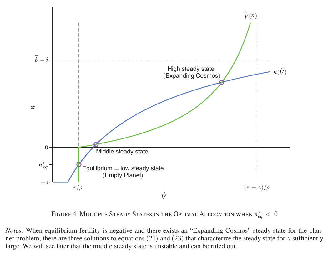
The picture that carries the paper is a plot of the two relations in $(\tilde V, n)$ space. One is the same for both allocations, $n(\tilde V) = \bar b - \delta - 1/\tilde V$, rising and concave. The other is the planner’s valuation:

which is eq. 21, p. 3505 in the log case: the planner values people above the household’s $\varepsilon/\rho$ only where population growth is positive, and is pinned to exactly $\varepsilon/\rho$ everywhere it is not. That vertical segment is the whole result. Two curves, one of them with a flat spot, cross three times: an Expanding Cosmos at high $\tilde V$ and high $n$, an unstable middle, and a low one at $\tilde V = \varepsilon/\rho$ with $n < 0$ that is simultaneously the decentralized equilibrium and a steady state of the planner’s problem. As Jones puts it at 00:16:00: “because of this kink that occurs at zero… the blue lines and the green lines intersect at three points… now the equilibrium, the empty planet result, is also a steady state of the planner’s problem.”

Note how odd that is on its own terms. The externality here is not small. Calibrate the model and see how not-small.

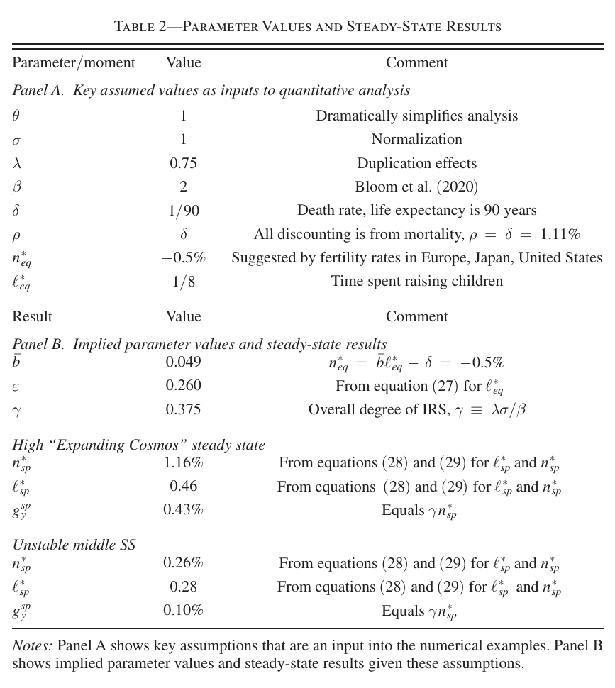
Equilibrium population growth is set to $-0.5$ percent, roughly Europe and Japan, with an eighth of a lifetime’s time spent raising children and life expectancy of 90 years. The implied optimum at the Expanding Cosmos is population growth of $1.16$ percent a year and forty-six percent of time devoted to children, delivering $0.43$ percent growth in income per person forever. That is an enormous gap between what happens and what a utilitarian planner wants — the planner would like the world to spend nearly half its waking effort having and raising children — and yet a planner handed the controls late enough will optimally decline to close it.

The deadline

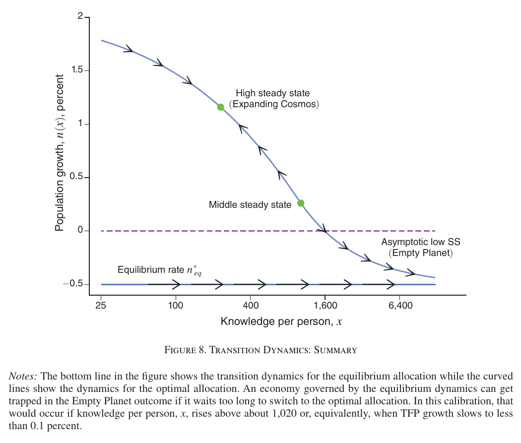
To see when, you need the dynamics, and here the log case earns its keep. With $\theta = 1$ the two-state problem collapses onto a single state $x \equiv A^\beta/N^\lambda$ — “knowledge per person”, ignoring the exponents, as Jones says — with the property that $\dot A/A = 1/x$. Optimal fertility turns out to depend on $x$ alone: more knowledge per head, less value in another head. And $\dot x = \beta - \lambda n x$, so $x$ rises whenever $n$ is negative or merely small (eqs. 24–25, p. 3508).

That last clause is the trap. Sit on the equilibrium path with $n = -0.5$ percent and $x$ drifts right, forever, at a speed you cannot influence by not deciding. Switch to the optimal allocation while $x$ is still low — at 100, or at 400, tfp growth of 1 percent or 0.25 percent — and the optimal path takes you left, to the Expanding Cosmos (p. 3513). Switch after $x$ passes the middle steady state and the optimal path also runs right, to the Empty Planet. In this calibration the door closes at $x^{*}_{middle} = 1{,}020$, that is, when tfp growth falls below 0.1 percent (p. 3514). Once even optimal population growth turns negative, at around $x = 1{,}600$, income per person rises a further 31 percent, ever (p. 3514).

This is Result 6, and it is the genuinely surprising thing in the paper — not the Empty Planet, which is arithmetic once $n < 0$. A reader coming in expects “delay is costly.” What they get is “delay changes which outcome is optimal.” The planner is not defeated, out-voted or budget-constrained; the planner does the sums again and decides the vanishing population is now the right answer.

What the talk adds, and where it differs

The 2020 video is Jones alone with slides for twenty-two minutes; there is no discussant and no audience, so there is nothing to report about what a room pushed back on. What the talk does is show which parts he thinks are load-bearing. He puts the kink up front, before any dynamics. He concedes the direction of the externality as a modeling choice, on camera, in a way the published version compresses into a citation. And he narrates the trap in causal words rather than in phase-diagram arrows: high $x$ means low $\dot A/A$ means low idea value of people, so “even the planner can have negative population growth,” and “if society delays adopting the good policies… even the planner can get trapped by the empty planet result” (00:21:06).

Two places where the talk is the earlier draft and should not be quoted at the published paper. First, the threshold: Jones says “if we wait till say x is 2000” (00:20:13); the published number is 1,020. Second, the character of the middle steady state. In the talk he describes it as “an unstable spiral… you actually never reach it… it’s called a [Skiba (1978)] point technically… you get this jump” (00:19:05, where the auto-captions mangle the name). That language is spoken only: the slide he is standing next to draws a continuous, if steep, $n(x)$, and the published baseline with $\ell^{*}_{eq} = 1/8$ gives a smooth schedule around a plain unstable source, with spirals and jumps demoted to footnotes and confined to lower $\ell_{eq}$ or higher $\gamma$ (footnotes 8 and 9, pp. 3509, 3512). The talk also runs only the log case; the published version carries generalized Barro–Becker throughout, adds a phase diagram and Results 4 through 6, and pushes the $\theta \ne 1$ multiplicity into an appendix.

What the paper concedes

More than you would guess. No demographic transition, no capital, no human capital, no quantity–quality trade-off, no urbanization, no rising female labour force participation (pp. 3497–3498, 3515–3516). The welfare criterion — dynastic utility of a representative generation — is one of several defensible ones, and with endogenous population the choice is known to matter. Knowledge depreciation is assumed away, and Jones notes that adding it at a constant rate makes things worse: not stagnation but decline. He names three escapes — automation and ai raising idea production enough to outrun the demography, mortality falling toward zero, evolutionary selection favouring high-fertility groups — and writes that “the results in this paper are not a forecast.”

My own reading, offered as such and not as the paper’s: everything here rests on $g_A$ being exactly zero when $n \le 0$. Any floor on idea production that does not scale with the number of living people — accumulated automation, ai, or simply more of the world joining the set of people who do research — keeps $z$ strictly positive, un-kinks the schedule, and can delete the low steady state altogether. The paper grants ai as a caveat in the conclusion but never shows what a small floor does to the multiplicity, which is the one comparative static a reader most wants. Relatedly, the deadline cuts both ways: tfp growth below 0.1 percent is an order of magnitude below anything currently measured, so on the model’s own calibration the door is not closing soon. And the baseline $\ell^{*}_{eq} = 1/8$ does quiet work, since a lower value produces the spirals the published figures do not show.

Still. The structure survives all of that, because the structure is not really about demography. It is about a corrective force that is proportional to the thing it is supposed to correct. Whatever you think of the calibration, a world with a positive externality that vanishes as the externality binds is a world where the standard advice — internalize it, subsidize it, get the prices right — has an expiry date, and where the honest recommendation is less “have more children” than “decide sooner.” Which, given that the deciding body is a planet’s worth of families each of whom is correctly indifferent between 1.9 and 2.1, is not so much a policy as a hope.

References