International Trade and Macroeconomic Dynamics with Sanctions

Fabio Ghironi (University of Washington, CEPR, EABCN, NBER), Daisoon Kim (NC State and NBER), Galip Kemal Ozhan (IMF and NBER). “International trade and macroeconomic dynamics with sanctions,” Journal of Monetary Economics 154 (2025) 103810, open access, twenty pages, of which the last two are references; the model appendix is online supplementary material rather than part of the article. The published version supersedes NBER Working Paper 32188 and cites it as its own earlier draft. The companion paper, “International Economic Sanctions and Third-Country Effects,” IMF Economic Review 72, 611–652 (2024), extends the same framework to a three-country world. No seminar recording could be found. PDF-only digest. The exhibits are cropped from the published PDF.

Ghironi–Melitz with a war in it

The sanctions on Russia after February 2022 were different in kind from every previous programme because the target was large — eleventh by GDP, a top energy supplier, a net creditor with the world’s fourth-largest reserves — and so the sanctioner could not pretend to be unaffected. What the paper builds is the open-economy DSGE in which that interdependence can be tracked quarter by quarter: Ghironi–Melitz (2005), the workhorse for trade with heterogeneous firms and endogenous entry in a dynamic general-equilibrium setting, with a commodity sector added and three kinds of sanctions that can be switched on. Western economies are Home, specialized in differentiated consumption goods made by heterogeneous firms that enter at a sunk cost and export above a productivity cutoff; the target is Foreign, specialized in a homogeneous intermediate — gas — produced by a fixed set of Cournot producers from labor and a natural resource. Home runs a surplus in consumption goods and a deficit in intermediates. Households trade bonds internationally subject to adjustment costs, so net foreign assets can be non-zero in the long run and initial positions matter. The mapping to Russia is direct, and the authors note it also fits China’s comparative advantage in homogeneous inputs against the US in differentiated goods.

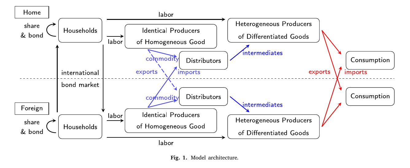
Three sanctions. Financial: a fraction of Foreign households is cut off from the international bond market and can only trade bonds with the unsanctioned Foreign households. Consumption-good trade: export or import bans that bite on the most productive firms — a second, higher productivity cutoff above which firms may not trade — a design the authors say is intended to capture the fact that sanctions primarily affect larger, highly productive firms, typically producing high-tech or advanced technology products. Commodity trade: a quantity restriction or price cap on Foreign’s gas.

The upper bar is the whole innovation. The ordinary export cutoff, call it $\underline{z}_{X,t}$, is still there, pinned down where export profits hit zero. The sanction clamps a ceiling $\bar{z}_X$ on top of it, so average exporter productivity and the number of exporters become

and setting $\varPhi(\bar{z}_X)=0.99$ puts the top one percent of firms out of the export market. Models that treat sanctions as tariff increases truncate the export distribution from below; this one clamps it from above, and the two have opposite compositional effects on who is left exporting. The published conclusion makes the point without the arithmetic, saying that treating sanctions as exclusion from markets is what distinguishes the framework from models in which “the adjustment to sanctions takes place primarily along the intensive margin of existing trade relationships.” The NBER working paper put it more bluntly, in a footnote that the published version cut: tariffs have the reverse compositional effect, excluding the lower-productivity exporters.

What moves the real exchange rate

The paper’s analytical section inherits Ghironi–Melitz’s exchange-rate decomposition, log-linearized as its Eq. (8):

Three channels: relative exporter productivity, the composition of the two consumption baskets, and the relative cost of effective labor and of intermediates, where $TOL^{Y}_{t}$ is the terms of labor in the consumption-good sector and $TOG_t$ the terms of intermediates. Read off it, the Home real exchange rate appreciates when Home’s effective consumption-sector labor gets dearer relative to Foreign’s, when Home’s intermediate input gets dearer, and when the average productivity of Foreign exporters falls (raising Home’s import prices); it depreciates when Home’s consumption basket shifts toward cheaper imports.

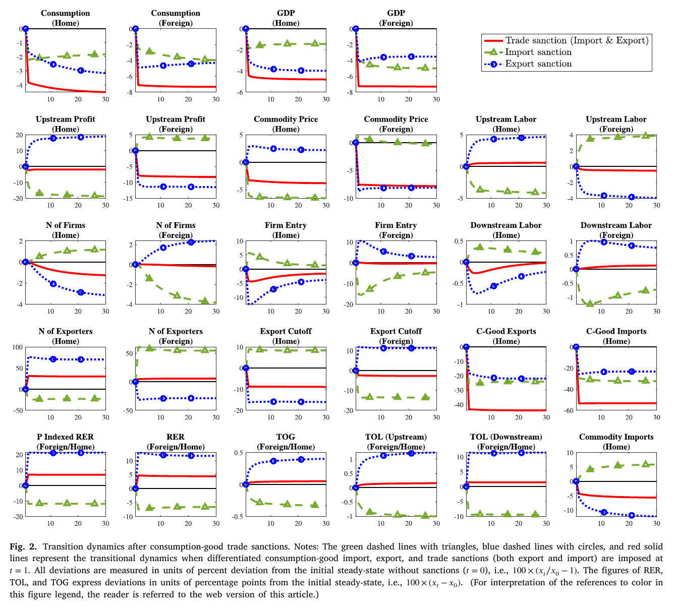
The sanctions then sort themselves by which channel they hit, and they emphatically do not all push the exchange rate the same way. An export ban on Home’s top firms makes entry at Home less attractive — a high draw no longer pays off in export profits — so entry shifts to Foreign, Home’s consumption-sector labor must become cheaper to keep the sector alive, and the Home real exchange rate depreciates; the lower export cutoff and the exclusion of the top firms both pull down average Home exporter productivity, reinforcing the depreciation. Import sanctions and financial sanctions run the same mechanism backwards. Both make Foreign the unattractive place to enter, entry shifts to Home, Home’s relative labor costs rise, and the Home real exchange rate appreciates. Financial sanctions reach that outcome by a route of their own: the sanctioned Foreign households take a wealth hit, cut consumption and therefore imports, which raises the threshold a Home firm must clear to be worth exporting and so lowers the average Home export price — but the sign is the same as under import sanctions. The commodity ban is the exception to the labor-cost channel, not to the direction of the move: cutting off Foreign gas forces Home to reallocate labor into commodity production and raises the relative price of Home’s intermediate so much that the intermediate-price term dominates the entry terms, and Home appreciates for a reason that has nothing to do with where firms choose to enter. Three of the four sanctions appreciate Home and only the export ban depreciates it, which is exactly the paper’s moral: “the exchange rate is not a reliable measure of the effectiveness of sanctions.”

Who pays, and the partial-sanctions result

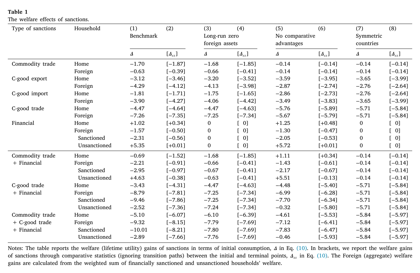
The welfare table is the paper’s contribution to policy. Every entry is a consumption-equivalent computed two ways, in Eq. (10):

— once along the transition and once by comparing the old steady state with the new one two hundred quarters out, and the wedge between them is a result in its own right. Sanctioning the target’s sector of comparative disadvantage hurts Foreign most and costs Home a great deal too, though how much depends on which way the ban runs: an export ban costs Home 3.12 percent of initial consumption against Foreign’s 4.29, both bans together 4.47 against 7.26, but an import ban on its own costs Home only 1.81 against Foreign’s 3.90, which makes it the one consumption-good sanction that is cheap for the sanctioner. Sanctioning the target’s comparative-advantage sector (gas) costs Home more than Foreign, 1.70 against 0.63, because Home has to reallocate labor into the commodity sector where it is inefficient. Financial sanctions alone make Home slightly better off, by 1.02, and hurt only the sanctioned Foreign households, while unsanctioned Foreign households gain 5.35 percent — they intermediate on behalf of the sanctioned ones, a windfall that survives only as long as the sanction stays financial, since under all three sanctions at once even they lose 2.89. That is the model’s version of the argument that partial financial sanctions on Russian banks are leaky: the sanction bites on Foreign aggregate consumption only when the sanctioned share is large enough that the unsanctioned cannot borrow and lend for everyone, so that entry finance dries up and the number of Foreign firms falls. Initial net foreign assets amplify financial sanctions through the wealth effect. The bracketed columns make the methodological point: steady-state comparisons overstate Home’s losses and understate Foreign’s, so welfare has to be computed along the transition. And comparative advantage is what gives sanctions their force on both sides — strip it out of the calibration and the combined-sanctions losses fall to 4.61 and 7.12 percent from the benchmark’s 5.10 and 9.32.

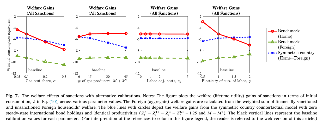
The robustness panels hold the paper’s genuine surprise. Short-run labor adjustment costs barely move welfare at all; the long-run elasticity of substitution across sectors moves it a lot, and in the wrong direction, since as long-run mobility rises Foreign’s losses fall but “Home welfare losses surprisingly increase.” The trap is that flexibility lets the pre-sanction Home economy specialize harder into differentiated goods, which is precisely what makes the forced reallocation hurt. At low mobility Home starts with 7.5 percent of its labor in commodities and ends with 8.8; at high mobility it starts with 3.7 and surges to 7.7. The gains from trade that mobility bought are the gains the sanction then destroys.

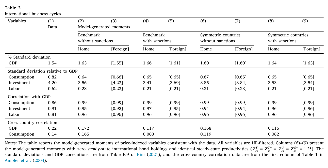
A last section looks at business cycles under sanctions and finds that they weaken international comovement and fragment markets but do not change the cyclical response to productivity shocks within each country. Cross-country correlations do collapse — GDP from 0.172 to 0.117, consumption from 0.165 to 0.083, against data of 0.22 and 0.14 — while the volatilities barely register the change, Home GDP going from 1.63 to 1.66. So sanctions desynchronize the world without making either half of it more turbulent, and on the model’s accounting they “would not create additional welfare costs through business cycle fluctuations.”

Where it sits

This is the “open-economy DSGE IMF stuff” the second Claude list named, and the paper that answers, within a fully dynamic model with two large interdependent economies, the question — which way does the exchange rate go under which sanction — that Itskhoki–Mukhin answer in a small-open-economy New Keynesian setting and that the block-2 sanctions empirics (Export Sanctions; dark shipping) answer with Russian microdata. Its value to the group is the machinery — Ghironi–Melitz is something a macro reader already knows how to extend — and two results that should be carried into the gotchas: sanctions on the target’s comparative-advantage sector are paid for by the sanctioner, and partial financial sanctions are largely undone by the unsanctioned. The published version is otherwise almost exactly the working paper, same calibration, same tables, same ten equations, but it did quietly drop the footnote gesturing at Clayton–Maggiori–Schreger-style strategic behavior, and those authors now appear nowhere in the text or the reference list, so the frontier the paper names for itself is a different one: the optimal choice of sanctions by sanctioning governments and of responses by targeted ones, the fiscal consequences for governments whose revenue depends on trade, and the role of central banks once nominal rigidity is added. That last item is the one to watch, and the paper says why in its own closing lines. Currency appreciation looks attractive to a central bank in a sanctioning country worried about sanction-driven inflation — and the paper has just shown that appreciation is the usual case — yet the same events that prompt the sanctions tend to produce downturns that call for easing. The exchange rate is not a scoreboard, and it is not a policy target either.