International Friends and Enemies

Benny Kleinman (Stanford and NBER), Ernest Liu and Stephen J. Redding (Princeton). American Economic Journal: Macroeconomics 16(4), 2024, pp. 350–385. Video: Liu presenting an early version at the STEG Theme 0 online workshop (CEPR/VideoVox), September 2020, about 33 minutes with a short discussion at the end; no discussant. The figures and tables below are cropped from the published version: Figure 4 and Figure 2, and Tables 1, 2, 3, 5 and 6.

Who gains when China grows

The question sounds like political science — do countries realign toward the partners they depend on economically? — but the contribution is a measurement that only a trade economist would make. “Dependence” is usually proxied by bilateral trade. That is wrong twice over: a country’s real income depends on its partner’s productivity through every other country’s trade costs, not just the bilateral ones, and productivity growth abroad moves the terms of trade in ways that can make a trading partner worse off. The paper’s move is to compute, from the full class of constant-elasticity trade models, the general-equilibrium elasticity of country $n$’s real income with respect to productivity growth in country $i$, for every pair, and to call $i$ an economic friend of $n$ if the elasticity is positive and an enemy if negative. Then it asks whether political alignment follows economic friendship, with two instruments. The panel is a balanced 143 countries over 1970–2012, with the trade elasticity fixed at $\theta = 5$ throughout (p. 362).

Enmity is not a rhetorical flourish; around 30 percent of bilateral pairs have it, though the negative values are small in absolute magnitude (p. 364). The typical enemies are raw-materials exporters competing for the same customers — Chile and South Africa, Saudi Arabia and Niger — and the probability of enmity rises when two countries do not trade directly at all, because then nothing is left but the cross-substitution effect. Which is the whole argument in one sentence: the bilateral flow you would have used as your dependence measure is precisely zero in the cases the model finds most adversarial.

The exposure matrix

In a single-sector Armington world with trade elasticity $\theta$, totally differentiating indirect utility and the market-clearing conditions gives the response of every country’s nominal and real income to a vector of productivity shocks:

(eqs. 10–11, p. 359), where $\mathbf{S}$ is the matrix of importers’ expenditure shares, $\mathbf{T}$ of exporters’ income shares, and $\mathbf{M}=\mathbf{TS}-\mathbf{I}$. Rearranging and inverting gives the object everything else rests on, the real income exposure matrix (eq. 12, p. 359):

with $\mathbf{Q}$ the stacked nominal-income vector that imposes world income as the numéraire. One matrix inversion, and you have the point elasticity for all $143 \times 143$ pairs. Note that $\mathbf{U}$ is not symmetric: $i$ can be your friend while you are its enemy.

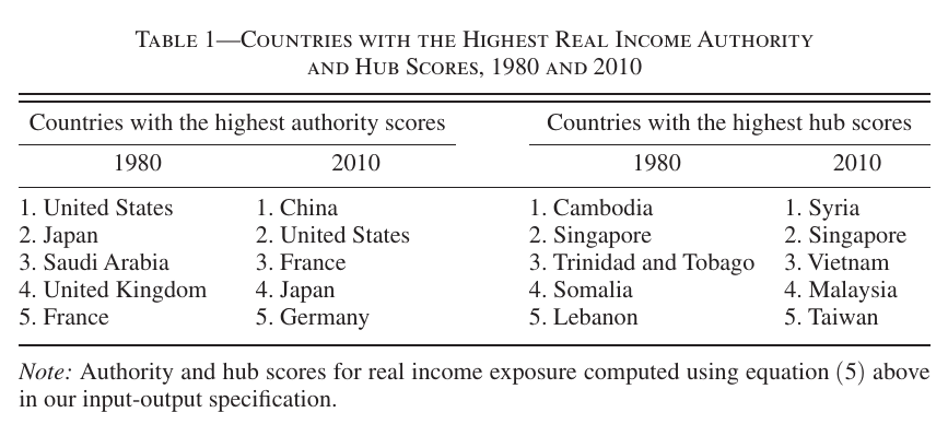
Stacked as a network, $\mathbf{U}$ yields authority scores — whose productivity growth moves the world — and hub scores — who gets moved (eq. 5, p. 358). The United States led on authority in 1980 and China leads in 2010, having been outside the top five thirty years earlier. Hubs are Cambodia and Singapore in 1980; Syria, Singapore, Vietnam, Malaysia and Taiwan in 2010. The scores are not just GDP wearing a hat: authority correlates with GDP at 0.66, hub at −0.10 (p. 366), and the residual variation is legible — countries deep in global value chains have authority above their GDP weight, commodity exporters below it.

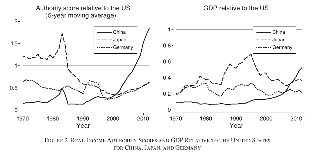
The sharpest descriptive fact is in Figure 2 (p. 367): the GDPs of Japan and China never exceed 70 percent of the US level between 1970 and 2012, and yet their authority scores comfortably exceed the American one, Japan’s in the 1980s and China’s in the 2010s. Being the country everyone’s real income depends on is not the same thing as being the biggest country, and the gap between the two panels is the paper’s case for bothering with the model at all.

A surprise Liu dwelt on in the talk: the linearization is nearly exact even for thousand-percent productivity shocks. The reason is charming. The nonlinear system takes logs of weighted averages and the linear one takes weighted averages of logs; the two coincide exactly under autarky and under free trade, and a real-world trade matrix is essentially a weighted average of the identity matrix (home bias) and the free-trade matrix (shares proportional to exporter size), plus residual noise that cancels inside a log average. “The world is a sphere,” Liu said, so distances between random pairs are noise — which is also, he noted, part of why gravity works so well. And they do not leave it at intuition: they bound the norm of the Hessian in the second-order term, which bounds every higher-order term too, and show the bound is tiny at observed trade matrices.

The China experiment

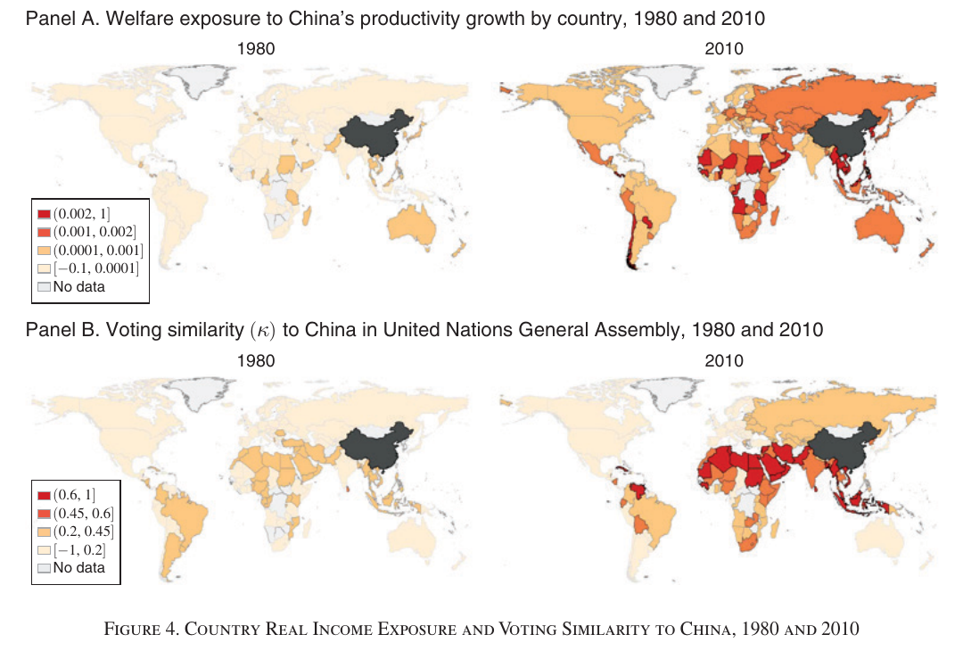
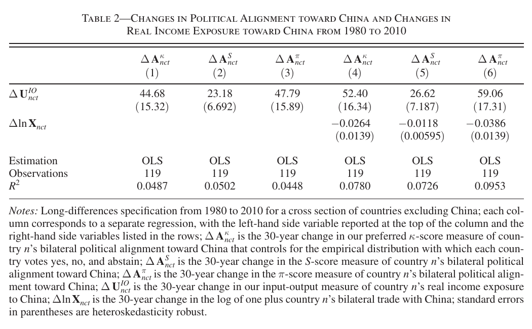
From 1980 to 2010, the countries whose exposure to Chinese productivity growth rose most — South-East Asia through regional production chains, resource-rich Africa and Oceania through the terms of trade — moved most toward China in UN voting. The OLS long difference on the preferred $\kappa$-score gives 44.68 (15.32), which the paper converts into the number worth carrying around: a one standard deviation increase in real income exposure to China buys a 0.26 standard deviation increase in political alignment toward China (p. 372).

Because exposure is an equilibrium object — and the paper’s own political model predicts feedback from alignment to productivity — it is instrumented. Start at the observed 1980 equilibrium, feed in an exogenous 100 percent increase in Chinese productivity computed by exact-hat algebra in the input-output model, hold everything else fixed, and read off the counterfactual change in each country’s exposure (footnote 17, p. 372). The pure supply-side prediction alone produces the realignment, and it produces more of it: the IV coefficient is 101.8 (27.78), roughly twice OLS, which the authors read as attenuation from high-frequency trade noise dominating the endogeneity bias. Political alignment, on this reading, responds to secular trends and not to the year’s shipping data.

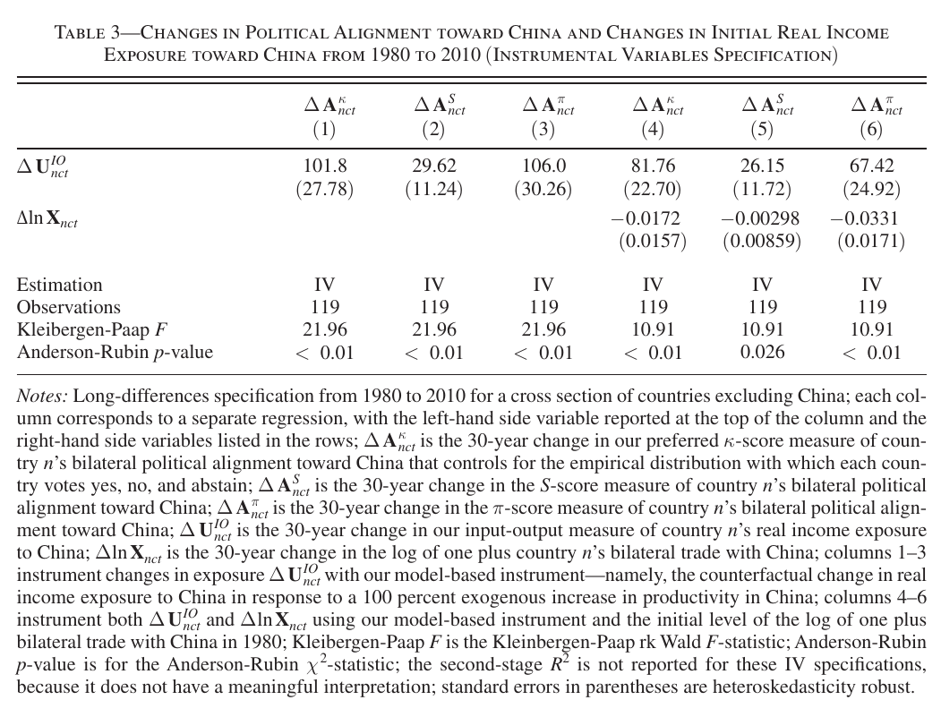
Bilateral trade with China is endogenous too, so where it enters as a control it is instrumented with its 1980 level, on the shift-share logic that the countries that gained the most trade with China are those already trading with China. The trade coefficient comes out negative — −0.0264 (0.0139) under OLS, −0.0172 (0.0157) under IV — while exposure survives at 81.76 (22.70). The paper is candid that log trade here is a reduced-form control on which the model makes no prediction. Still, if you had been planning to use bilateral trade as your proxy for economic dependence, note that it enters with the wrong sign.

The air-travel experiment

The second instrument follows Feyrer: land masses make sea distance and air distance diverge sharply for some pairs, so as air freight got cheap the short-air, long-sea pairs gained disproportionately, and that geography does not move. The implementation detail matters, because it is the paper’s own reason the two instruments differ (p. 377). Exposure is instrumented from a sectoral gravity equation with time-varying coefficients on log air and log sea distance, whose fitted expenditure shares are pushed back through equation (12), so the instrument inherits general-equilibrium feedback and sectoral heterogeneity. Bilateral trade is instrumented from an aggregate gravity equation, which carries only the direct effect. The second stage has exporter-importer, exporter-year and importer-year fixed effects, so the exporter-year terms absorb the sign and magnitude of the exporter’s productivity growth and what is identified is the elasticity.

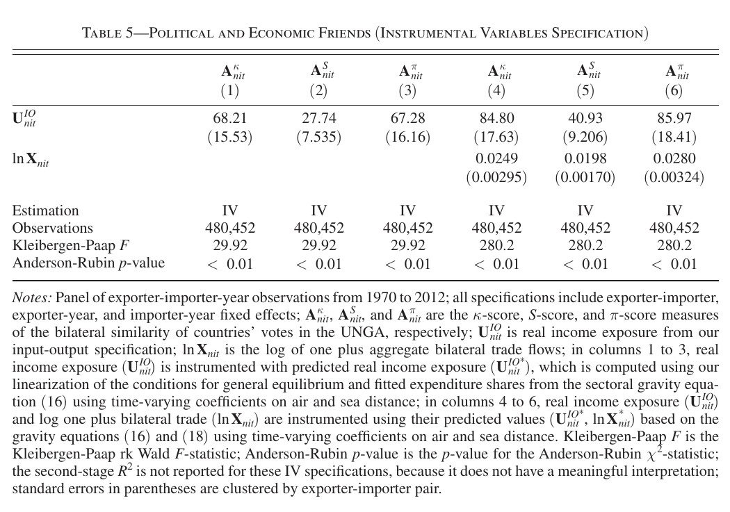
The headline is 68.21 (15.53) on 480,452 exporter-importer-year observations, again about twice the OLS 24.79 (3.955), implying that a one standard deviation rise in real income exposure raises bilateral political alignment by 0.094 standard deviations (p. 379). The first stage has power — a Kleibergen-Paap F of 29.92, with Anderson-Rubin p below 0.01 — though it is worth noticing that this is the one diagnostic that got worse on re-estimation for publication, down from 33.69 in the working paper. Everything else moved in the comfortable direction.

The comparison that matters for the group is in columns 4–6, and it is more interesting than the version one might expect. Adding instrumented log bilateral trade does not leave the exposure coefficient alone: it rises, from 68.21 to 84.80 (17.63). And log trade is not statistically absent — its coefficient of 0.0249 (0.00295) is more than eight times its standard error, about as precisely estimated as anything in the paper. It is simply economically minute: doubling bilateral trade with a partner moves the voting-similarity score by roughly 0.017. So the honest statement is not that trade does nothing, but that trade is measured precisely enough for us to be confident it does almost nothing, while the theory-based measure does the work and gets stronger once trade is held fixed. Bilateral trade is not a good proxy for economic dependence; it is a good proxy for bilateral trade.

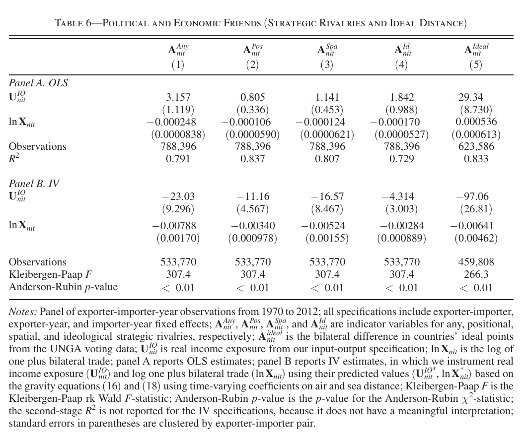
The same design runs through the other political outcomes, and there the results hold on nearly every measure rather than on every one. Exposure reduces the propensity to be strategic rivals — −23.03 (9.296) for any rivalry under IV — shrinks the ideal-point distance from the US-led liberal order, −97.06 (26.81), and raises the propensity to hold a formal alliance, 16.81 (6.419). Two cells break the pattern, and the paper flags both itself. Ideological strategic rivalry is insignificant under IV, −4.314 (3.003), though larger in absolute value than its OLS counterpart, so the failure is in the standard error rather than the point estimate. And neutrality pacts are insignificant under OLS, 0.992 (0.992), becoming significant only under IV at 11.68 (5.813), with an Anderson-Rubin p of 0.1; the authors suggest neutrality is a decision about all your neighbours at once rather than about any one of them, which is a fair thing for a bilateral regression to struggle with. The alliance data are worth a moment on their own: in 2010 China had four allies — Iran, North Korea, Russia and Pakistan — the United States had 49, and the median country had 10 (p. 364). A validation exercise rounds it out, showing that the exposure measures detect the jump in interdependence when preferential trade agreements are signed, with no pre-trends and robustness to the staggered-adoption estimators.

What was asked

The discussion was brief and produced three questions, collected before Liu answered any of them. The chair asked how different the patterns would look with service flows in them. Liu’s answer was that this is a toolkit rather than a model — whatever flows you observe, the same algebra applies, and non-tradables just rescale the measures by their expenditure share — before conceding what the paper actually does, which is “something quite crude”: take the US services share and scale all the welfare measures by it.

Berthold asked the question that produced the best answer: why does a linear approximation survive China, which we usually think of as a very large change, and is it really a sequence of small steps? Liu declined the escape route — even a single thousand-percent shock is fine — and gave the autarky-plus-free-trade decomposition and the Hessian bound, adding that it had surprised the authors too. Finally David asked, explicitly as clarification and not criticism, whether aggregate exposure hides the within-country winners and losers that make trade with China politically fraught. Liu answered that the multi-industry version gets at exactly that, though the paper does not push it: if employment is sticky by sector, the cross-industry exposures are the object you want, and the contrast is enormous. A uniform Chinese productivity gain helps East Asian electrical and medical equipment through regional production chains while destroying textiles and office equipment; for commodity exporters it runs the other way, with basic metals, mining and agriculture expanding as light manufacturing dies. He called it Dutch disease in general equilibrium.

Where it sits

This is the empirical hinge between blocks 1 and 2: the block-1 gravity papers use alignment as the regressor and trade as the outcome, this paper reverses the arrow and shows alignment responding to a model-based measure of who gains from whom. Its motivating model — countries pay for actions that raise partners’ productivity in proportion to their own exposure — is a Nash game in gifts, with no threats available to anyone in it, which makes it the benevolent twin of Liu–Yang’s International Power, where the same toolkit is turned to measuring who can hurt whom. Read the two together; the exposure matrix here and the power measure there are built from the same expenditure shares and the same elasticity and answer opposite questions. Whether the country that can hurt you and the country you vote with are the same country is, mercifully, not something this paper has to decide.