Why Are the Wealthiest So Wealthy? New Longitudinal Empirical Evidence and Implications for Theories of Wealth Inequality

Joachim Hubmer, Elin Halvorsen, Sergio Salgado and Serdar Ozkan · forthcoming, Econometrica; circulated as St. Louis Fed Working Paper 2024-013 · read from the draft of 10 July 2026 · no recorded talk, so everything below comes from the paper itself

The average Norwegian household had net worth of about $434,000 in 2019. A household in the top 0.1% aged 50 to 54 had 124.3 times that. The interesting question is not that the number is large; the interesting question is which line items got it there, and until recently nobody could answer that with data, so the literature answered it with models. You nominated a mechanism — the rich earn more per krone, or the rich are more patient, or the rich inherit, or the rich briefly earn superstar wages — you calibrated it until it reproduced the observed top wealth share, and you declared the mechanism plausible. Everyone knew this was a weak test. This paper is what happens when you finally get to run the strong one.

The whole paper is one accounting identity, and Norway lets you fill in every term but one

You are a household. Each year you begin with some net worth, you receive capital income on it, you receive labour earnings, and occasionally somebody dies and you receive an inheritance, or somebody generous is still alive and you receive a transfer. You spend some of that and keep the rest. So:

Here $W_{i,t}$ is household $i$’s net worth in year $t$, $R_{i,t}$ the return on net wealth (including unrealised capital gains, and net of interest payments and of wealth and capital income taxes), $L_{i,t}$ after-tax labour earnings including self-employment income and transfers, $H_{i,t}$ inheritances and inter vivos transfers net of tax, and $S_{i,t}$ the gross saving rate out of total resources — eq. (1), p. 8. This is not a theory. It is a bank statement, and it is true by construction.

The Norwegian registers fill in most of it directly: bank accounts, bonds, mutual funds, listed shares, personal debt, labour earnings, interest, transfers and taxes are all third-party reported. Some of it is imputed instead, and the paper is candid about which — housing values annually from a machine-learning model on contemporaneous transactions, owner-occupied housing income at about 2.2% of property value, pre-2005 dividends and capital gains by gradient boosting trained on the post-2005 shareholder registry, post-2013 inheritances by giving each child an equal share of the estate. Unlisted equity is carried at tax values, which the paper notes “correlate highly with book values, which generally exclude intangible assets and may understate true economic values.” Pension wealth, offshore wealth, art and jewellery are out.

One term is never observed at all, and it is consumption. Nobody has a register of what Norwegians ate. So the saving rate is not measured; it is the number that makes the identity balance given the other four. Which means “saving rate heterogeneity,” the paper’s headline finding, literally means “the residual left over after we accounted for returns, wages and inheritances,” and you should hold that thought, because it is the sharpest thing anyone can say against the paper and the authors get there before you do.

Higher saving rates, then inheritances, then returns, and labour barely shows up

To decompose, you take the identity, iterate it forward, and notice that the entire wealth path is a function of five objects: where you started, and then four sequences.

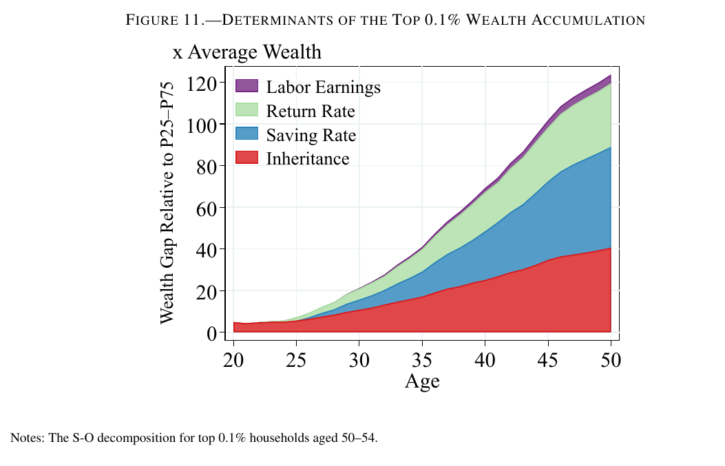
$f$ is the forward iteration of the identity from initial wealth $W_{i,1993}$, and $\bar R_t$ is the return of the reference group — the middle 50%, households between the 25th and 75th percentiles of wealth in the same cohort and conditioning year — so the second expression is the counterfactual in which the top 0.1% keep everything about their lives except that they earn mid-wealth returns (unnumbered displays, p. 18). Do that one factor at a time and the answers are enormous: give the top 0.1% mid-wealth returns and terminal wealth falls from 124 to 31 times average wealth; give them mid-wealth initial wealth at 20 and it falls by about 85; give them mid-wealth saving rates and it falls by a staggering 115. Labour is worth about 9. Inheritances received after age 20 are worth only about 21, which is the paper’s quiet knife: what matters about a transfer is less its size than how many years of compounding it gets (p. 19).

Those numbers add to well over the whole gap, because the identity is jointly nonlinear — high returns matter less once you have taken away the large inheritances they were compounding — and because the order of removal changes the answer. So the paper averages each component’s marginal effect over all 120 orderings of the five factors, a Shapley–Owen decomposition, which has the property that the pieces sum exactly to the gap. For the top 0.1% aged 50 to 54 the pieces are saving 39.1%, inheritance 32.8%, return 24.7%, labour 3.4% (p. 20). Averaged over terminal ages 45 to 64 the abstract rounds this to 36 / 31 / 28 / 5, which is the same object, not a competing estimate.

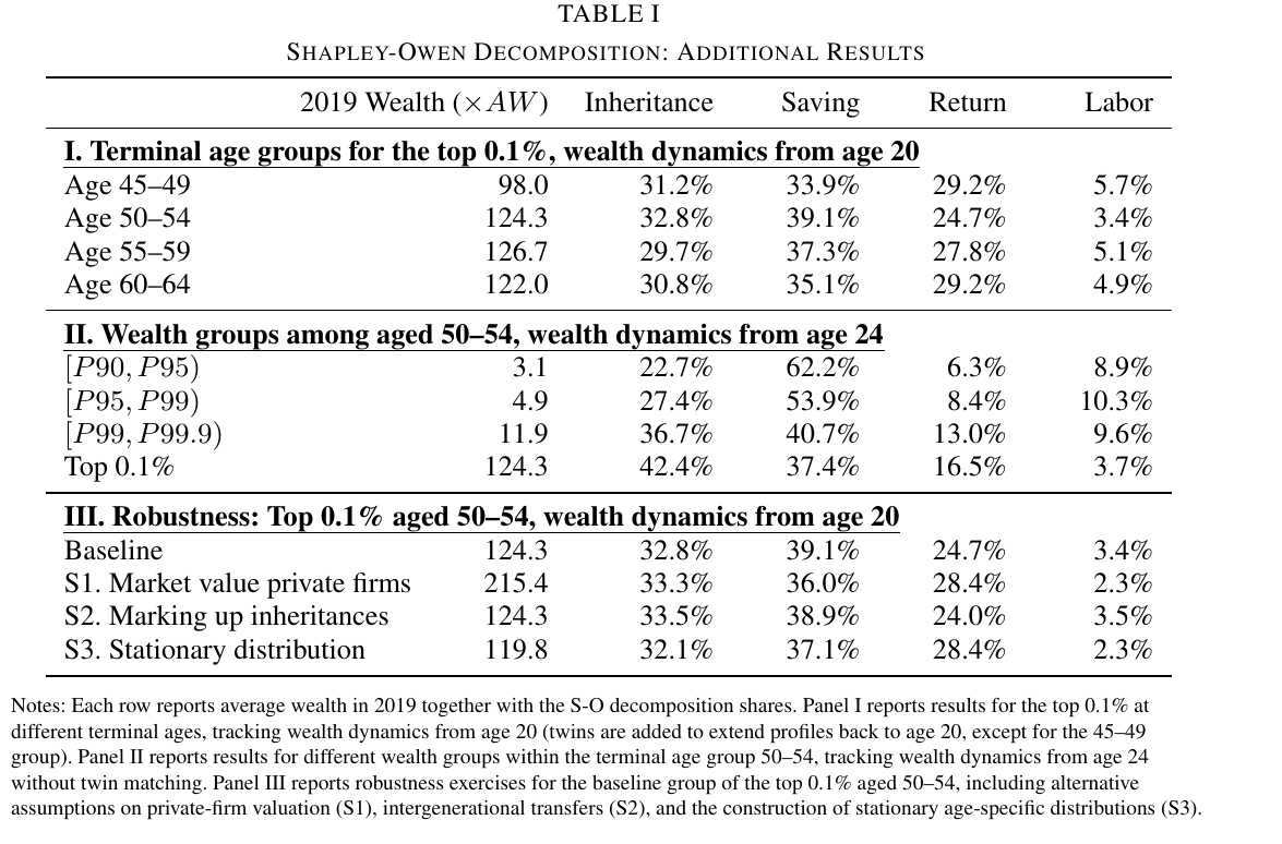
Two things to take from Table I. Climbing the top decile, inheritance rises from 22.7% of the gap at P90–P95 to 42.4% at the very top and returns from 6.3% to 16.5%, while saving falls from 62.2% to 37.4% and labour rises to 10.3% before collapsing to 3.7% at the top; ordinary affluence is a saving story, and great wealth is not. And the levels are fragile while the shares are not: mark private firms to market with listed-firm multipliers averaging about 1.8 and terminal wealth nearly doubles, to 215.4 times average wealth, but the shares move only to 33.3 / 36.0 / 28.4 / 2.3, “because initial wealth, capital income, and savings all rise roughly proportionally.”

Worth saying plainly what these households are, because it governs everything after. They are not portfolios. Equity is 85 to 90% of the top 0.1%’s holdings, above 90% on a 26-year average for the benchmark group, and almost all of it is private business; leverage runs about 50% of total assets, essentially all of it inside their firms, since direct household leverage excluding firm liabilities is 1.8%. Below the 90th percentile, housing is about 90% of gross wealth. So the “return on wealth” of the rich is mostly the operating performance of a company they run, and the “saving rate” of the rich is mostly earnings their company retained.

New Money earns twice the return of Old Money, on the asset it owns less of

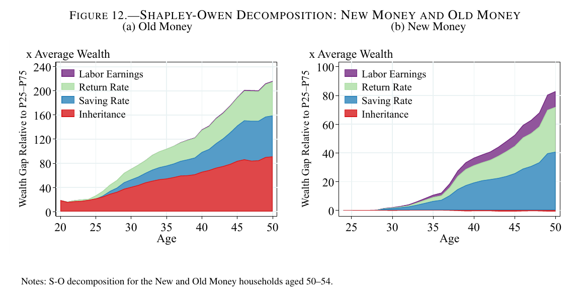
The average of the top 0.1% is a composite of two populations, so the paper splits the group into quartiles by initial wealth plus the present value of all future net inheritances, and names the bottom quarter New Money and the top quarter Old Money. By construction that is a quarter each; independently, 24.0% of the top 0.1% at 50 to 54 were already in the top 0.1% in their mid-20s and about 24% started below the 90th percentile, so the labels are not artefacts of the cut.

Old Money begin their early 20s at 25.9 times average wealth and end at 217.0. Their starting wealth is not earned: summed post-tax labour earnings to age 24 come to 1.19 times average wealth, 4.6% of what they already had, or 3.8% if you capitalise it at their own later saving and return rates. Their decomposition is inheritance 42.2%, saving 31.4%, return 25.9%, labour 0.6%. New Money begin at minus 0.1 times average wealth — 9.5% of the portfolio in equity and a debt-to-asset ratio of 1.47, which is how you get there — and end at 83.7, with 95.4% of their portfolio in private business. Their decomposition is saving 50.1%, return 37.6%, labour 13.3%, and inheritance −1.1%, negative because they started poorer than the middle-class households they are being compared with.

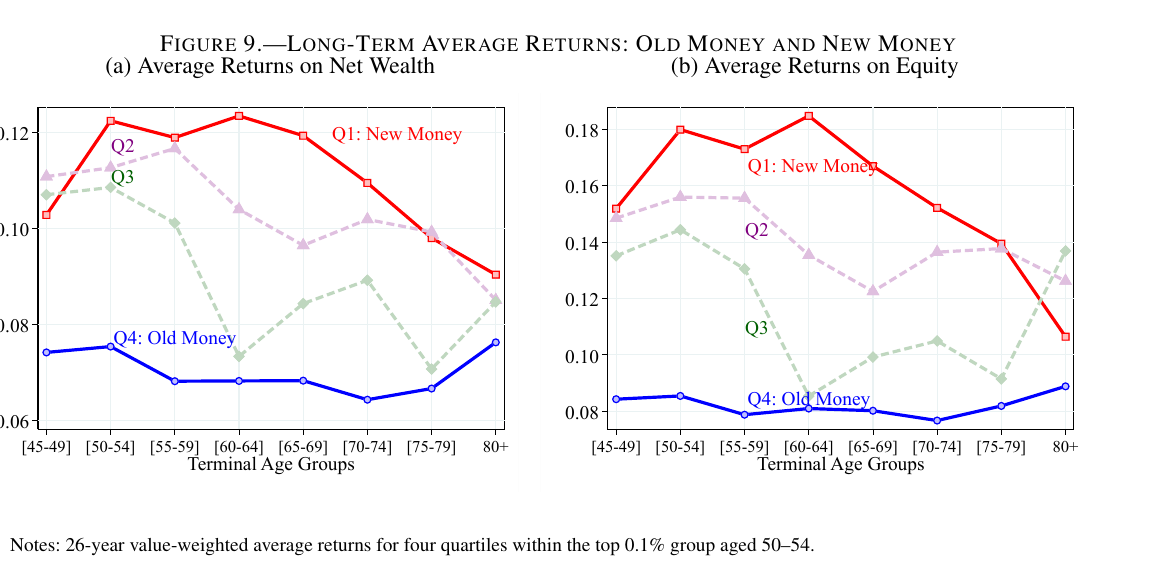
And here is the surprising thing, which is a fact about returns and not about any model. Everyone who has read the returns literature expects returns to rise with wealth, and across the whole distribution they do: among 50- to 54-year-olds the 26-year average return on net wealth climbs monotonically from 1.4% below the median to 9.1% at the top. But that gradient is composition. Returns on equity are hump-shaped — about 12% below the median, above 16% in the top 10%, back down to about 11% for the top 0.1% — so the very rich do not out-pick, they out-allocate. And inside the top 0.1% the sign flips outright: New Money, who hold less equity and hold it later, earn 18.0% a year on equity against Old Money’s 8.5%, and 12.2% against 7.5% on net wealth. The households with the least capital earn the most per unit of it, which is either a puzzle or, if you have ever met a decreasing-returns-to-scale production function, a diagnosis.

The friction is a collateral constraint, and it bites hardest on the productive poor

Before the paper builds that model it disposes of five others, and this is the methodological punch. Take the basic lifecycle Bewley economy with Norwegian taxes, Norwegian mortality and a non-Gaussian Norwegian earnings process, and it fails the cross-section outright, generating a top 0.1% wealth share of 0.8% against 9.3% in the data. Now add, one at a time, a superstar earnings state, fixed heterogeneity in returns, heterogeneity in the discount factor, and a nonhomothetic warm-glow bequest motive. All four hit the top wealth share. Two of them also hit the top income share. On cross-sectional evidence all four are alive, which is exactly the situation the literature has been in for thirty years.

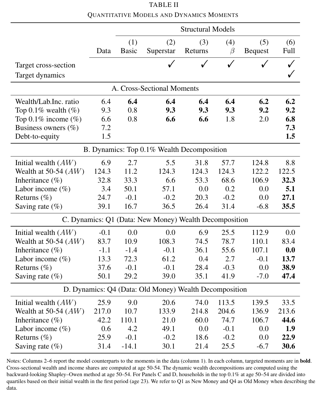
Then run the same backward decomposition on each model’s own simulated households, and they fail — but they fail in different directions, which is worth being precise about. Against the data’s 32.8% inheritance share, the returns model gives 53.3%, the stochastic-discount-factor model 68.6%, and the warm-glow bequest model 106.9%, with a saving contribution of negative 6.8% because its wealthy heirs run their inheritances down. Return contributions in those models are essentially nil. The three of them also start the top 0.1% far too rich — initial wealth of 31.8, 57.7 and 124.8 times average wealth against 6.9 in the data — and their bottom quartiles richer still, at 6.9, 25.5 and 112.9 against the data’s −0.1. In the paper’s phrasing they “produce too few self-made households”: not none, too few. A model nominally about return heterogeneity turns out, dynamically, to be an inheritance model wearing a returns costume, and you could not have known that from the cross-section.

The superstar model is the partial exception, and the paper says so, calling it the closest to New Money dynamics. It starts its top group poorer than the data, at 5.5 against 6.9, and its bottom quartile starts at zero and climbs to 108.3 times average wealth on a labour contribution of 61.2% with inheritance at −0.1%. That is genuinely the right shape. It just gets there the wrong way: labour and returns together account for 56.9% of the top gap against 28.1% in the data, inheritance only 6.6%, and its Old Money never compound, ending at 133.9 against 217.0. Its rich people are paid rather than invested, and its heirs are inert.

So you need two ingredients. The first is returns that rise with productivity but fall with scale, which is what a decreasing-returns technology behind a borrowing limit delivers. The second is a reason for the already-rich to keep saving hard when their returns are only moderately good.

$w$ is net worth, $k$ entrepreneurial capital under the collateral constraint $k\le\lambda w$, $z$ a fixed entrepreneurial type correlated with permanent labour ability and persistent across generations, $\zeta$ an i.i.d. shock, $\mu=0.8$ the returns-to-scale parameter, $\delta+r$ the user cost and $c_f$ a fixed operating cost; the second term of the utility function is wealth itself, and crucially it is not multiplied by the death rate, so unlike a bequest motive it makes people save hard while they are young (unnumbered equations, p. 27). A talented person with little wealth can only operate $k=\lambda w$, which is far less capital than her productivity wants, so her profit per krone of net worth is enormous and she grows fast; an established fortune has all the capital it can profitably use, and $\mu<1$ means the next krone earns less than the last. New Money and Old Money fall out of the same technology at different points on it.

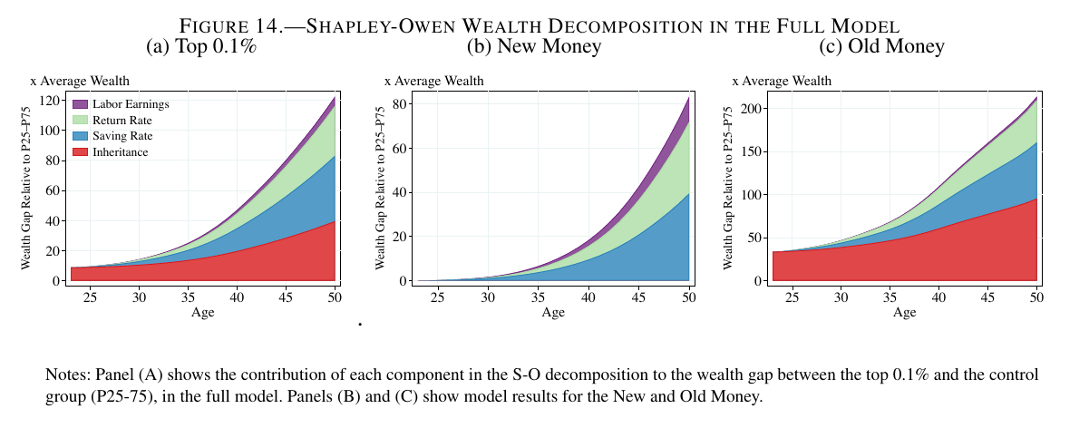
Nine parameters, fourteen moments. The fit is close: top 0.1% wealth share 9.2% against 9.3%, income share 6.8% against 6.6%, business owners 7.3% against 7.2%, debt-to-equity 1.5 against 1.5, and a top-group decomposition of 32.3 / 5.1 / 27.1 / 35.5 against the data’s 32.8 / 3.4 / 24.7 / 39.1. But be careful how you read Figure 14, because the paper is careful too: all three decompositions are targets. The paper says it disciplines the mechanisms “by directly targeting our dynamic S-O decomposition facts,” $\rho_{ez}=0.473$ is tied to the New Money labour contribution and $\rho_z=0.721$ to the Old Money return contribution, and every decomposition share in that column is printed in bold. The model matching the paper’s central fact is fit, not prediction. What is genuinely untargeted is where each group’s wealth profile starts and ends — New Money from 0.0 to 83.4 against −0.1 to 83.7, Old Money from 33.5 (data: 25.9) to 213.6 against 217.0 — and with fourteen moments and nine parameters, five of the targets function as over-identifying restrictions in any case. That is a real achievement and a modest one, and conflating it with prediction would be doing the authors no favours.

The objections, which are mine rather than a discussant’s

There was no seminar recording, no discussion and no Q&A attached to this draft, so what follows are the sharpest challenges I can construct, each with what the paper itself says.

The first is the residual. Saving is defined by the identity, not measured, and the returns it is defined against are built partly from imputations. Hold measured wealth changes fixed and any error that inflates measured capital income mechanically lowers the inferred saving rate — the krone amount saved does not move, implied consumption rises to absorb it — and the headline result is precisely that saving beats returns, 39.1% to 24.7%. The paper identifies exactly this channel for undervalued inheritances and fixes it by reversing the statutory discounts (70% on private equity below NOK 10m until 2009, 40% after, an inferred 45% on real estate), and the adjusted series then matches heirs’ share of donors’ end-of-life estates, which is decent validation. It also reports a saving rate defined out of cash on hand with similar conclusions. What it does not do, and does not claim to do, is apportion measurement error between $R$ and $S$.

The second is what a private Norwegian firm is worth. Top portfolios are overwhelmingly private business, carried at tax values that track book values and may omit intangibles, in a country that levies a wealth tax on those values — which is a standing incentive for them to be low. Worse, the plausible mismeasurement is heterogeneous in exactly the dimension under study, since a fast-growing start-up’s book value understates its market value far more than a mature firm’s does, and that is precisely New versus Old Money. The paper’s answer is the market-value robustness exercise, which doubles the level and leaves the shares alone, and it notes that the multipliers are an upper bound because listed firms are positively selected and that firms above roughly $500,000 in revenue are audited. But the multiplier is applied uniformly, so the differential version of the objection is not answered.

The third is selection. Conditioning on who ended up in the top 0.1% conditions on an endogenous outcome, and backward-looking returns and saving rates flatter the lucky by construction: 18.0% is the realised history of eventual winners. The paper concedes the point in a footnote on its second page and names the survivorship bias, then answers it with a forward-looking design sorted on initial wealth, where saving rates still rise from 25–30% below P75 to as much as 80% at the top, “though the relationship is quantitatively weaker,” where returns are still persistently higher for those who start rich, and where the top 0.1% of 20- to 24-year-olds show no mean reversion at all, going from 18.8 to about 40 times average wealth by their mid-40s. Two defences the paper leaves on the table: the same backward procedure is applied to the model-simulated households, so the selection is symmetric across data and models, and the quantitative gap between the backward and forward saving gradients is never reported in the main text.

The fourth is the one I find sharpest, and it is about when the clock starts. Age-20 wealth is folded into the inheritance category, on the reasonable ground that wealth at 20 essentially is a transfer. Track the same households from age 24 instead, without the twin-matching that extends profiles back to 20, and the inheritance share goes from 32.8% to 42.4% while returns fall from 24.7% to 16.5%, “because all initial wealth at age 24 is interpreted as inheritance.” So “inheritance is about a third” and “inheritance is about 42%” are the same data under two defensible conventions, both printed in the same table, and the paper does not foreground the tension. It does defend the underlying interpretation with the Old Money earnings calculation, and it does show the shares barely move across terminal ages 45 to 64, which is a different kind of stability.

The fifth is Norway, a small rich country with over 80% homeownership, tax policy that favours both housing and private business, a wealth tax, an inheritance tax abolished in 2013, and public pension funds owning roughly a third of domestic public equity. The paper flags all of it, notes that pensions are excluded because more than 80% of them are pay-as-you-go, cites an estimate that hidden offshore wealth would add about a percentage point to the top 0.1% share, observes that unlike the American evidence highly educated professionals neither dominate top wealth nor drive the New–Old Money difference (partly, it suggests, because of public health care and a civil-law tradition), and points out that the US Survey of Consumer Finances shows the same lifecycle decline in wealth concentration. Reasonable, and still not a claim that the shares would replicate in Houston.

And

The findable moral is that a cross-section is a photograph and these people needed a film. Four models that agreed about the photograph turned out to disagree completely about what happened before it, three of them insisting on a slow multigenerational drip that the Norwegian registers say is only about a third of the story, one insisting on a spectacular salary. The less findable moral is about the word “returns.” Two decades of work has treated the high returns of the rich as a fact about investors, which invites the thought that some people are simply better at picking assets. On this evidence the very rich are not better pickers — their equity returns are lower than the merely rich — they are people whose wealth is a company they operate, and the eye-watering 18% belongs to the ones who had a good business and not enough money to run it properly yet. Which is a sentence a venture capitalist would recognise instantly, and which took an entire national tax registry to establish.