Tapping into Scientific Talent: The Rise of Corporate and Public R&D in Japan's Chemical Industry

Takuya Hiraiwa (University of Maryland, Robert H. Smith School of Business), sole author. Presented by Takuya Hiraiwa at the nber Economics of Talent Conference, Cambridge ma, 2 October 2026 (video). No discussant. Paper version: the August 11, 2026 draft.

In 1913 Jōkichi Takamine (adrenaline; top of the first applied-chemistry class at the Imperial College of Engineering; in the United States since 1890) addressed the Chemical Society of Japan and complained that his country had trained nearly 2,000 university chemists and given them nothing to do. Hiraiwa uses the speech, in English translation, as the epigraph of the paper:

Thus, there are already people with the potential to invent. However, they are just busy with their jobs and lack the time to invent and innovate. Even if they come up with some kind of ideas, there are no funds to test them, and no required equipment in factories.

The next year Europe went to war. Japan barely fought, but its advanced chemicals came from Germany and Britain, and now they mostly didn’t. Chemical imports collapsed relative to domestic output, prices soared, and firms poured into the industry; the paper puts chemical-sector gnp growth at 35 percent a year during the war. Then imports came back, and close to 100 firms exited in 1920–24, about two-thirds of the wartime entry.

So you have something close to a four-year prohibitive tariff that nobody had to vote for, landing on a stock of trained chemists who had been waiting for one, almost all of whom you can name. Hiraiwa asks two things. When the demand for new chemistry arrived all at once, which of those chemists could actually supply it? And why did the invention keep going after the demand went away? (The talk opened with a modern case: Jian-Ping Wang’s rare-earth-free magnet research at Minnesota predated the 2010 Chinese export controls that made it urgent.)

Who answered

The data are a census of chemistry-related graduates of the four Imperial Universities from 1877 to 1930: 2,462 people in the paper, though the slide’s cohort counts add up to 2,474 (1,018 + 1,456). Graduation lists come in rank order, alumni registers give each year’s employer, and patents (the universe of roughly 126,000 to 1940) and papers in Japan’s two top chemistry journals are linked to each graduate. The treated group is the 620 chemists who had graduated by the eve of the war: 192 had published in those journals before 1915, and 428 had not.

The design is an individual-level difference-in-differences, with mechanical and electrical engineers as the control group, so that whatever the Second Industrial Revolution was doing to all high-tech graduates is differenced out (paper p. 19):

Here $y_{it}$ is patent applications by graduate $i$ in year $t$, $\mathrm{WWI}_t$ covers 1915–19, $\mathrm{PostWWI}_t$ covers 1920 on, $\mathrm{Chem}_i$ marks the chemistry divisions, and $d_i, d_t$ are individual and year fixed effects. The sample is graduates up to the 1914 cohort.

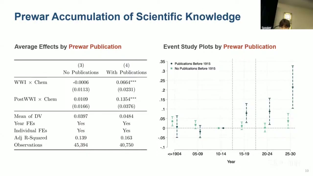
Pooled, the chemists patent more during the war and more again after it. Split by pre-war publications, the pooled effect comes apart. Chemists with the same degree and no publications have a wartime coefficient of −0.0006 and a postwar one of 0.0109. Neither is distinguishable from zero. Chemists who had published got 0.0664 during the war and 0.1354 after it, so the postwar effect is about twice the wartime one. The paper scales these against a mean of the dependent variable, 0.0484, and calls them “2.4 times” and “almost four times” the baseline. The table notes don’t say how that mean is built, so treat the multiples as rough. The event study is flat before the war, apart from one slightly positive early bin for the no-publication group.

The paper calls what the publishers had “embodied scientific knowledge”, and its reading of the case histories is that they mostly did not patent the topic of their old papers. Yoshikawa’s caustic-soda process was not anticipated by his 1898 and 1900 papers. They drew, the paper says, on “the totality of their accumulated scientific human capital”. The war did not reward the chemist who happened to be holding the right project. It rewarded the one who had been doing science at all.

Publications, or just the better students?

The obvious worry is that a publication just marks the best students. Publishers did rank higher and more often held doctorates (Table A.2). Hiraiwa splits the sample both ways, and the talk summarised the result as “publication record still matters even after controlling” (05:27:18).

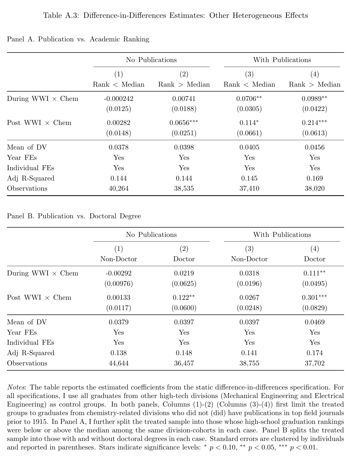
For the wartime response the claim holds up. In every cell without publications the wartime coefficient is about zero, including the above-median-rank students (0.00741) and the doctors (0.0219). The postwar period is less tidy. Students with no publications and above-median rank show a postwar effect of 0.0656***. Doctors without publications show 0.122**. Publishers without a doctorate show nothing in either period (0.0318 and 0.0267). The paper’s text flags only that last null. So the defensible version is narrower than the slide. Publications pick out who could respond to the shock; once the war is over, a doctorate predicts a lot of the persistence on its own, and “publications, not credentials” is the wrong summary of the postwar half.

Why it outlived the war

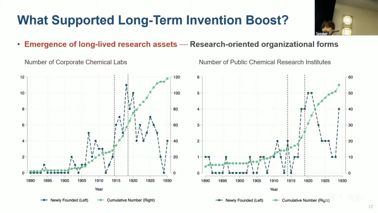
The war also left behind buildings. Read off the slide, the cumulative count of corporate chemical labs went from about 30 in 1914 to about 120 by 1930, and public chemical research institutes from about 15 to about 55, with foundings lagging the corporate labs by a few years: Riken in 1917 (which, the paper notes, grew directly out of Takamine’s speech), the Osaka Industrial Research Institute in 1918, an Army lab in 1919 and a Navy institute in 1923. The share of chemistry graduates in research rose from about a quarter to more than a third in the 1920s, and note for later that the research sector includes the Imperial Universities themselves.

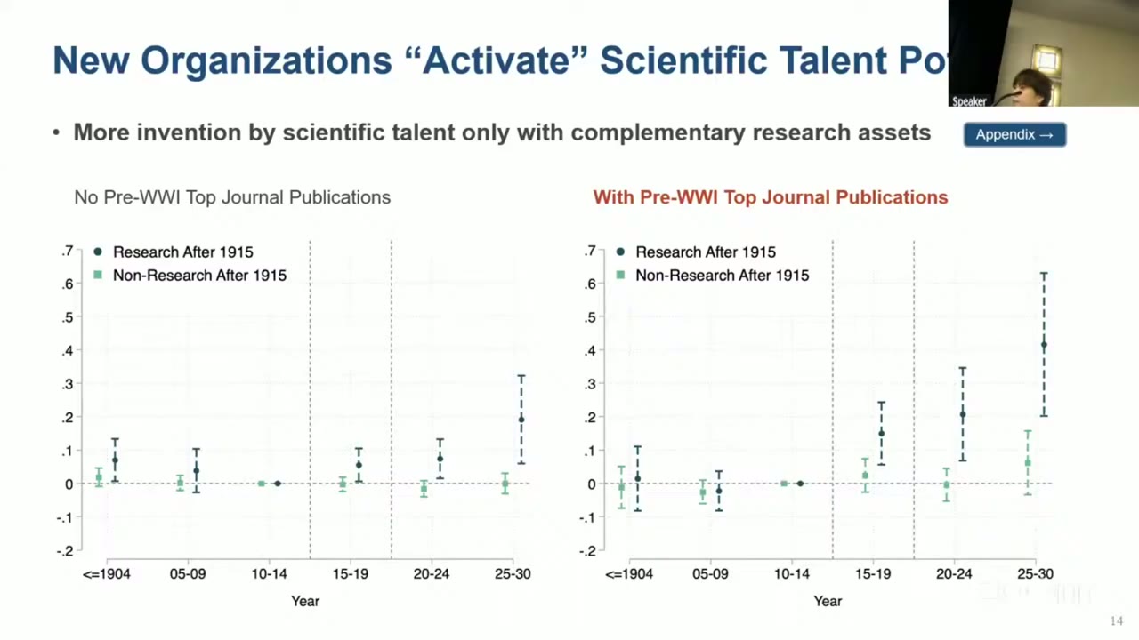
Split the publishers by whether they ever took a research job and the postwar boom sits almost entirely with those who did. The ones who stayed in production or teaching look like engineers. Hiraiwa was franker about this on stage than the paper is: “I want to be clear that this is just a result of selection … it’s kind of the description of where you can find the postwar invention boom … but still it’s informative about mechanism” (05:30:47). The paper says the same figure “helps to rule out” a general-trend story, which is a fair use of it. It does not rule out that the chemists most eager to invent were the ones who went to labs. The left panel shows the selection: the no-publication chemists who later took research jobs are already a little above zero before the war.

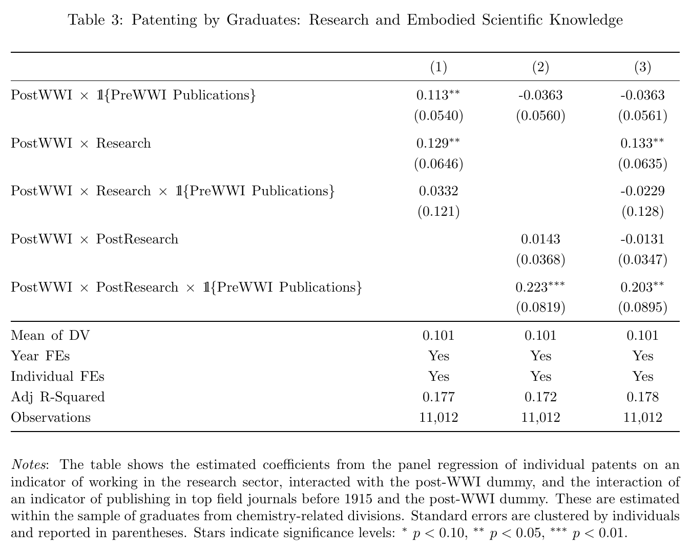
Table 3, which wasn’t in the talk, is the most interesting result in the paper. While someone holds a research job, the postwar boost is about 0.13 whether or not they published, and the triple interaction is indistinguishable from zero. The difference comes when they leave. Coding a dummy for every year after a person’s first research job, only publishers keep the boost after moving back into industry (0.223***), and publications on their own drop to −0.036. With only the current research job controlled (column 1), publications alone still carry 0.113**, and the paper concedes that at that stage “it may seem like” embodied knowledge had an independent effect. The reading: the lab is equipment anyone can use while inside it, and the trained scientist takes something with him when he leaves. Two cautions. Nobody was randomly moved, and since the “research sector” includes the universities, “publisher with research experience” partly means “chemistry professor”. There are 192 publishers in total.

Where the patents went

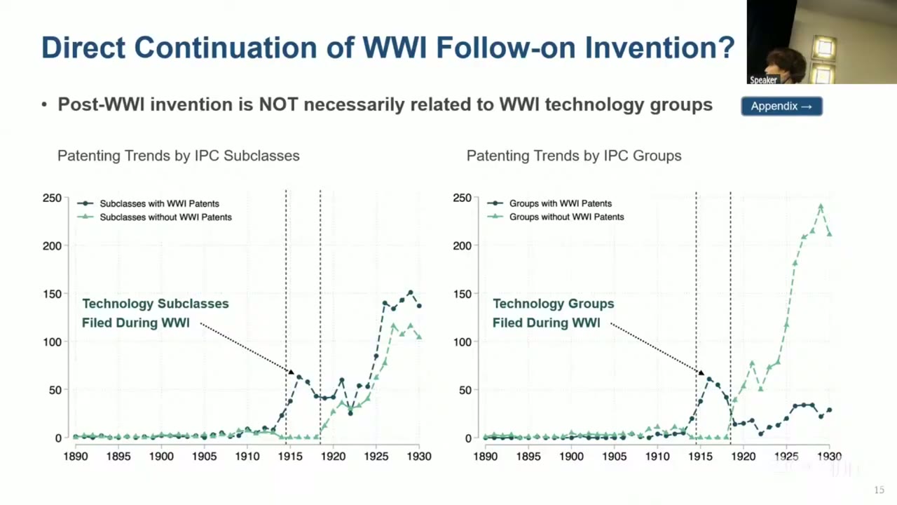
The surprising result is this. If the war’s legacy were learning by doing in import substitutes, postwar patents should pile up in the technology groups where wartime patents were. They don’t. At the ipc-group level, groups with wartime patents peak around 60 in 1916 and fall back after the war. Groups that had no wartime patents at all climb to about 240 a year by 1929. The demand shock asked for substitutes for specific imports. The lasting invention mostly went elsewhere. (These are counts in levels, which more graduates after 1919 inflate on both lines; Table A.4 does it per person.) Hiraiwa’s point is that neither directed technical change nor the infant-industry argument predicts this, since both send later invention down the path the shock opened.

The model: wartime problems as stepping stones

The model is in Appendix E. It got about a minute of the talk, introduced with “obviously I don’t have enough time to explain all the detail of the model” (05:32:55). It is uncalibrated and makes no quantitative contact with the coefficients above; its job is to say how a temporary shock could send invention somewhere new. In the Callander (2011) and Carnehl–Schneider (2025) setup, questions are points on a line and the true answers are one fixed realisation of a Brownian path. Knowing the answers at nearby points sharpens your guess at a new one: between two known points the conjecture variance is a Brownian-bridge arc that is zero at each end, and beyond the outermost known point it grows linearly. The core is eqs. (3)–(5):

Here $\mathcal{Q}_t$ is the set of domestic discoveries, $\mathcal{Z}$ the foreign technologies, $\delta_0$ the novelty threshold, $\lambda$ the reward, $\sigma_x^2(Y\mid\mathcal{F}_{jt})$ agent $j$’s conjecture variance at $x$ given what $j$ knows, and $c(\rho)$ a convex cost of success probability $\rho$ with $c'(0)=\underline c$.

The whole argument depends on where $\mathcal{Z}$ enters. A foreign technology appears in the novelty term but not in the variance term: an import at $z$ makes any domestic answer near $z$ worthless, but nobody in Japan knows how it was made, so it sharpens nobody’s conjecture. Foreign technology is all business-stealing and no spillover. Research pays only where variance is below $\bar\sigma^2=\lambda/\underline c$ and novelty is at least $\delta_0$. Under condition (7), every question cheap enough to attempt lies within $\delta_0$ of something already known or imported, and research stops for good (Prop. 1(iii)). The paper’s main text says foreign technologies “can stifle” domestic research, which is the right modal verb, because (7) is a condition, not a theorem about Japan in 1913.

The war takes the triangles away. Questions in the bands $\mathcal W$ around the missing imports now earn a scarcity premium $p$, with novelty judged only against domestic discoveries (eq. 11), so research restarts next to the missing imports. Scientists know every domestic discovery and non-scientists know only their own ($\mathcal F_{Nt}\subseteq\mathcal F_{St}$), so scientists’ variance is weakly lower and their success probability weakly higher: $\rho^*_{Nt}\le\rho^*_{St}$ (Prop. 2(iii)). The inequality is weak, and the main text glosses it as research “predominantly conducted by scientists”. The data’s −0.0006 is sharper than the theorem.

The postwar result needs an assumption, eq. (12), the hypothesis of Prop. 2(ii):

Here $\bar z$ and $\underline z$ are the outer edges of the foreign set and $t_1$ is the last war period. The condition says wartime discoveries got as far as the edge of the foreign set. Given that and $\delta_0<\min\{\lambda,p\}/\underline c$, condition (7) fails forever, no postwar discovery falls in $\mathcal W$ (Cor. 1(i)), and almost surely all but finitely many later discoveries lie beyond the foreign set, with the frontier diverging (Cor. 1(ii)). That is Figure 7B in a sentence. The import substitutes are stepping stones, and the postwar invention happens on the far bank.

So the model does not derive that four years of war were enough to get across; it assumes it. Whether Japan’s stepping stones reached the edge is the empirical question, and the evidence for it is Figure 7B, the fact the model was written to explain. (The proofs, in Appendix F, I have not checked.) The organisational extension, in which institutes lend non-scientists the scientists’ knowledge only while they work there, is verbal only, which is a pity, since it is exactly the Table 3 pattern.

Q&A

There was time for one question. An unnamed questioner asked what directions the postwar patents took: into fields where the English or Germans already were? Hiraiwa answered that Japan’s patent system, like the American one, required novelty, so the patents had to be distinct from German or English technology, “more domestic new technology area” (05:35:08). That answer rests on the patent examiner more than on the data. Asked whether they also patented in the us, he said some did, visible through Google Patents, “around the 10% of the patenting” (05:35:43). He said foreign filing could serve as a quality measure, and that he hasn’t built it yet. The 10 percent is from the talk only; the paper does not report it.

Takamine’s 1913 diagnosis was that Japan had the chemists and lacked the labs and the money. The paper’s answer, a war later, is that he was right on both counts: the chemists who had kept doing science were the ones who could respond, and the labs were what made the response last. It took a temporary emergency to build the permanent thing he had asked for, and one of the first institutions built was Riken, whose founding the paper traces directly to his speech.

References