Consumption Strikes Back? Measuring Long-Run Risk

Lars Peter Hansen, John C. Heaton and Nan Li, Journal of Political Economy 116 (2), April 2008, pp. 260–302. Published version. No seminar recording or discussant; John Heaton explains the paper in a four-and-a-half-minute Chicago Booth interview from 2012.

The consumption-based asset pricing model has a famous problem, which is that consumption barely moves. Take quarterly consumption growth seriously as the thing investors fear and the covariances are tiny, so the risk premia are tiny, and the risk aversion needed to fix that is absurd; this has been known since the early 1980s, partly thanks to Hansen himself. Since then most of finance has priced risk with factors made out of returns instead, and consumption got demoted to a footnote in the introduction. This paper is the attempt to bring it back, which is where the title comes from. The pitch is that the model was not wrong about consumption. It was looking at the wrong horizon.

Heaton puts the idea in plain terms in the interview: measuring investors’ well-being by “the quarter-to-quarter movements in consumption or gdp” is “too narrow a view” (00:01:47). If you lose your job today, your consumption dips a little now, “but my whole future looks a lot different” (00:02:15). A shock that moves today’s consumption by a little and the whole future path by a lot is a big shock, and a quarterly covariance will not see most of it. So the paper asks a different question from the usual one. Not “what is the one-period risk-return trade-off?” but “how is exposure to macroeconomic risk priced in the long run, for cash flows far in the future?” It then measures the answer and applies it to the value premium.

There is a second, quieter motive, and it is the more interesting one. The authors say outright that stylized models like theirs are misspecified “when examined with full statistical scrutiny” (p. 261): habits, durability, transaction costs and behavioural noise all mess with the high-frequency implications. You can patch each of these with an ad hoc transient term, or, in their phrase, “accept the misspecification and seek to decompose the implications.” The long run is where the transient junk washes out. So the long-run trade-off is not only interesting; it is the part of the model you might actually be able to believe.

The mechanism: a capm for the far future

The setup is deliberately linear. A state vector follows a var, $x_{t+1} = Gx_t + Hw_{t+1}$, with standard normal shocks $w$. Log consumption growth and the log stochastic discount factor are both linear in the state and the shock. A cash flow is a geometric random walk with drift, $D_t^* = \exp(\zeta t + \sum_{j\le t}\pi w_j)$, times a stationary transient factor $f(x_t)$ that can be anything you like. The vector $\pi$ is the cash flow’s long-run exposure to each shock, and the whole paper is about assigning a price to it.

Pricing a claim to $D_{t+j}$ means applying a one-period valuation operator $j$ times, and the value of a far-off payoff decays toward zero at some asymptotic rate $\nu$. Finding that rate is an eigenvalue problem: the operator has a strictly positive eigenfunction $e(x) = \exp[U_s(I-G)^{-1}x]$ with eigenvalue $\exp(-\nu)$ (Result 1, p. 267; the appendix formalises this as a change of measure, following what became Hansen and Scheinkman 2009). Subtract off the long-run growth rate of the cash flow, $\eta = \zeta + \tfrac12\pi\cdot\pi$, and what is left is the long-run rate of return:

This is Theorem 1 on p. 268: $\varsigma^*$ is the long-run return on a cash flow with no long-run exposure (a discount bond, say), $\pi$ is the exposure, $\pi^*$ is the price of long-run risk built from the discount factor’s shock loading $\xi_0$, and $\nu$, the gap between return and growth, doubles as a Gordon-growth measure of duration.

That is a capm, just evaluated at infinity: the long-run expected return is a riskless rate plus price times quantity. The nice part is what drops out. The transient factor $f$ and the drift $\zeta$ affect the value of the cash flow but not the long-run risk price. And the same is true of the discount factor: habit models and social-externality models that differ from the baseline only by transient terms change the eigenfunction $e$ but not the eigenvalue (Sec. II.E), so they share the same long-run trade-off. This is the formal version of “accept the misspecification.” You can be agnostic about a whole zoo of short-run stories and still say something about the long run.

Now plug in preferences. The representative investor has Epstein–Zin (1989) recursive utility with risk aversion $\gamma$ and, in the baseline, a unit elasticity of intertemporal substitution, which makes the continuation value log-linear in the state and everything else tractable. The discount factor’s loading on the shocks becomes

from p. 276 (and p. 264), where $\lambda_0$ is the impact response of log consumption to the shocks and $\lambda(\beta)$ is the $\beta$-discounted sum of all future responses. The second term is the continuation-value channel: under recursive utility, news about future consumption is priced today. That is the Bansal and Yaron (2004) mechanism, and, measured with consumption rather than the market return, it is Campbell and Vuolteenaho’s (2004) “bad beta” (p. 264).

The long-run price that comes out of this is

where $\lambda(1)$ is the undiscounted long-run response of consumption (p. 269). For $\beta$ close to one these are approximately the same. This is a slightly deflating observation for anyone who thought the Epstein–Zin versus power-utility fight was about the long run. In the limit the two preference specifications price long-run risk identically; recursive utility earns its keep in the short-run prices, by charging for predictability up front. Either way, the long-run price of risk is risk aversion times how far consumption eventually moves. Which means the entire empirical question is: how far does consumption eventually move?

Measuring the long run, which is the hard part

To answer that, the authors run a bivariate var (five lags) in log consumption of nondurables and services and log corporate earnings, both from the nipa, quarterly 1947 to 2005 (p. 280). Earnings are there because they predict consumption: “Changes in corporate earnings signal changes in aggregate productivity, which will have long-run consequences for consumption” (p. 278). The load-bearing assumption is that consumption and earnings each have a unit root and are cointegrated one for one: they “grow together,” responding identically to permanent shocks in the long run (p. 279). Shocks are normalised in the Blanchard–Quah (1989) spirit, so that one shock is temporary (no long-run effect on either series) and one is permanent, and by design the permanent one dominates long-run valuation (exactly under power utility, approximately under recursive utility, fn. 16). Compare Bansal and Yaron, who infer the slow-moving component as a latent variable from consumption alone; here it is pinned down by an observable series and a cointegration restriction (fn. 13).

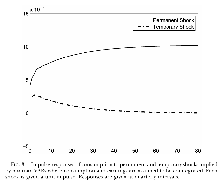
Fig. 3 is the long-run risk in one picture. The permanent shock moves consumption on impact by roughly twice what the temporary shock does, and then keeps going: the response “ultimately accumulates to a level that is more than twice the on-impact response” (p. 280). Most of the risk arrives after the quarter in which a covariance would look for it.

Then comes the honest part, which the paper does better than most. Long-run responses are extrapolations from a finite var, and they are estimated much less precisely than impact responses (the impact response converges at the parametric rate, the long-run response at a slower one, fn. 18).

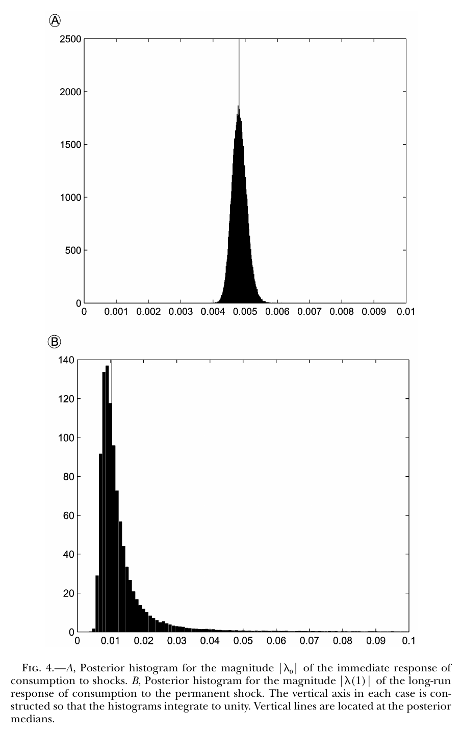
Fig. 4 shows the posterior for the size of the impact response, a tight spike around half a percent, and for the long-run response, centred around one percent with a right tail stretching past five. Note the horizontal axes differ by a factor of ten. The data are confident about what happens this quarter and quite relaxed about what happens eventually.

The specification matters too.

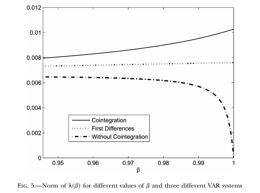
In Fig. 5, the cointegrated system gives the largest $|\lambda(\beta)|$. A var in first differences is lower and flat. A var in log levels without cointegration is estimated to be stable, so its long-run response is exactly zero, and for moderate $\beta$ it cuts $|\lambda(\beta)|$ by about a third (pp. 283–284). In other words, whether consumption has any long-run risk in it at all is, at the margin, a modelling choice, and the one the authors make is the one that gives a bigger answer. They say so: the restriction “ensures a larger value of $|\lambda(\beta)|$ and hence larger risk prices for any given value of $\gamma$” (p. 284).

How big is the answer for consumption itself? Small. For a claim on aggregate consumption the long-run excess return is $\lambda(1)\cdot[\lambda(1)+(\gamma-1)\lambda(\beta)]$, and at the point estimates $\lambda(1)\cdot\lambda(1) = 0.0001$, so even with $\gamma = 10$ the premium is 0.4% a year ($10 \times 0.0001 \times 4$, p. 284). That is the equity premium puzzle (Mehra and Prescott 1985) again, at a longer horizon. But the posterior gives a 10% chance that it exceeds 1.65% a year, against 0.4% for the short-run counterpart, and the authors’ summary is carefully worded: “A notable price for long-run risk cannot be ruled out by these data once a large value of $\gamma$ is assumed.” Cannot be ruled out. Consumption has not struck back yet; it has filed a motion.

The evidence: value stocks own the long run

The real application is to the cross-section. Sort stocks into five book-to-market portfolios, from growth (portfolio 1) to value (portfolio 5), and build each portfolio’s dividend series from its returns with and without dividends, smoothed over four quarters to remove seasonality (p. 288).

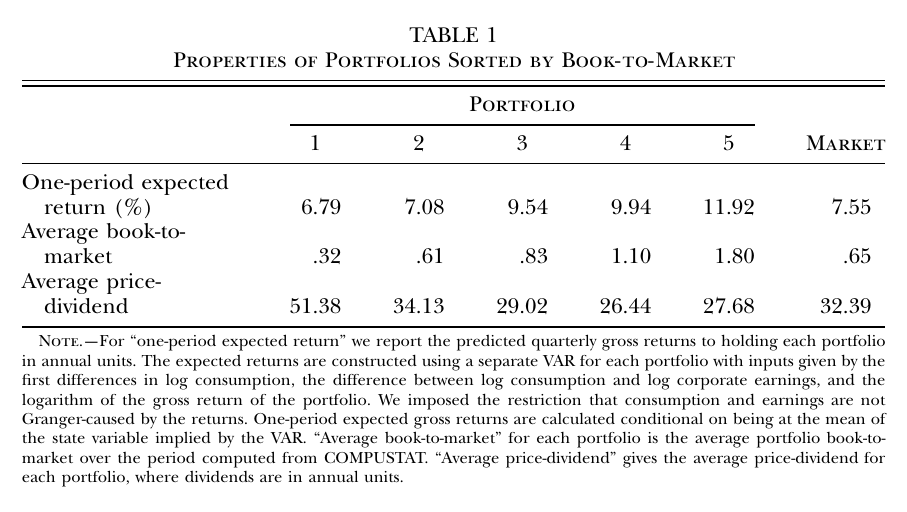
Table 1 is the puzzle being explained: one-period expected returns, predicted from a var with the state at its mean, climb from 6.79% for growth to 11.92% for value, and it is “well documented” that contemporaneous consumption covariances cannot account for that (pp. 287–288).

To measure each portfolio’s exposure, the authors add its log dividends to the consumption–earnings var as a third variable, with a third, orthogonal dividend shock that is allowed a permanent effect of its own (dividends get their own stochastic growth component; they are not cointegrated with consumption). Then they do a Beveridge–Nelson (1981)-style martingale decomposition of dividend growth. The loading of the martingale component, $\iota(1) = \iota_0 + U_d(I-G)^{-1}H$, is exactly the $\pi$ of Theorem 1 (p. 286). Long-run exposure is the long-run impulse response of log dividends.

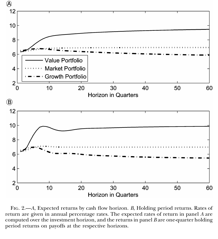
Fig. 2 is the paper’s money shot, with $\gamma = 20$ (fn. 7: “This large value is used to amplify the effects of risk”). Price each portfolio’s cash flows one horizon at a time. At short horizons value, growth and the market all sit around 6.5% a year; “the risk premia for all portfolios are similarly small for short horizons” (p. 271). Then they split. The expected return on value cash flows rises toward 9.5% at fifteen years, growth drifts down below 6%, and the market sits around 7%. The limits are good approximations after about two years (p. 272).

The pivotal number is the exposure, and here the paper is admirably upfront about precision.

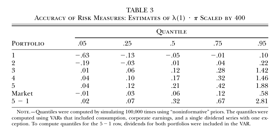
Under unit elasticity of substitution the long-run expected excess return is approximately $\gamma\lambda(1)\cdot\pi$, so Table 3 reports the posterior for $\lambda(1)\cdot\pi$, scaled so you multiply by $\gamma$ to get annual percent. Growth’s median is $-0.05$, slightly negative: in the long run growth dividends are, if anything, a mild consumption hedge. Value’s median is 0.21. The value-minus-growth row, estimated in a var with both dividend series, has a median of 0.32, a 5th percentile of 0.02 and a 95th percentile of 2.81. The authors’ reading is “significant evidence that the cash flows of a portfolio of value stocks are riskier than those of the portfolio of growth stocks” (p. 293), and that is fair: the sign is robust and the magnitude is not. (A bracketing remark of my own, not the paper’s: at $\gamma = 20$ the 5–1 posterior median implies a long-run spread of about 6.4% a year, and the point-estimate limiting rates in Table 2 below give 9.92 − 5.39 = 4.5%; the observed one-period spread is 5.1%. These are different horizons, and the paper never equates them or backs out a $\gamma$.)

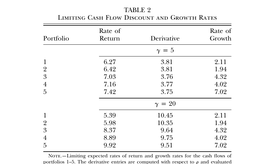
Table 2 adds the duration side, and it is where the model starts to creak. Value dividends grow much faster in the long run (7.02% a year against 2.11% for growth), yet growth stocks have the higher price-dividend ratios. Gordon growth with a common discount rate gets that backwards; the model can square it only if growth stocks’ long-run discount rate is much lower, which requires a sizable $\gamma$ (pp. 291–292). At $\gamma = 5$ and unit elasticity, value’s duration measure $\nu$ is 7.42 − 7.02 = 0.40 percentage points, “barely positive,” and “even small increases in $\beta$ or reductions in $\rho$ make this measure negative, implying an infinite price-dividend ratio” (p. 292). At $\gamma = 20$ the gap opens to 2.90 for value against 3.28 for growth. The authors also flag that Table 2 is “likely to be fragile from the standpoint of measurement accuracy.” Risk aversion, here, is doing double duty: generating the premium and keeping the value portfolio’s price finite.

The one surprising thing

The value premium, in this accounting, lives almost entirely in the long run. In priced terms, value and growth look alike at short horizons: “The short-run exposure is similar to that of portfolio 1, but the long-run exposure is much higher” (p. 291), and Fig. 2’s strips start together. The difference opens up only after a couple of years, when value dividends keep accumulating their response to a permanent consumption shock and growth dividends do not. That is a clean explanation of why a one-period consumption-capm test fails on this cross-section: it is measuring covariance in the window where the two portfolios are most similar. It is also an uncomfortable explanation, because the window where they differ is exactly where Fig. 4 and Table 3 say the data are least informative. The risk is real to the extent that you trust the extrapolation, and the extrapolation is the thing you can least check.

Weak points, mostly the authors’ own (no discussant exists)

There is no discussion or Q&A to report; the Booth interview is a lay summary of the motivation and does not discuss the portfolio results. But the paper is unusually forthcoming about where it is soft, and the sensitivity analysis is part of the contribution rather than a robustness appendix.

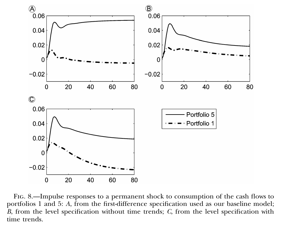
First, the cash-flow growth specification. Fig. 8 re-estimates the dividend responses under three ways of modelling dividend growth: the baseline (a separate stochastic growth component), a levels model where consumption and earnings are the only source of growth, and a levels model with a deterministic time trend, close to Bansal, Dittmar and Lundblad (2005). For each portfolio the three specifications agree for about twelve quarters and then diverge “in ways that are quantitatively important” (p. 295). Value’s long-run response is around 0.05 in the baseline and around 0.02 in both alternatives. Growth’s is slightly negative in the baseline, slightly positive without a trend, and clearly negative with a trend, which would make growth stocks a substantial long-run consumption hedge. The value-minus-growth gap is roughly the same in the baseline and the trend model, which is the consolation. The authors reject the trend model on economic grounds (deterministic trends “known a priori to investors” seem unlikely, and Sims warns that trends overfit initial conditions, fn. 24) and keep the baseline, which they call, fairly, “ad hoc” (p. 296). That is a reasonable call, but it is a call, and the limit you get depends on it.

Second, $\gamma$. The headline figures use $\gamma = 20$, which is a lot. The authors offer a reinterpretation via Anderson, Hansen and Sargent (2003): the change of measure buried in the recursive-utility discount factor can be read as investors’ concern that their model is misspecified, so $\gamma$ measures doubt rather than risk aversion. They then ask how hard it would be to detect that misspecification. With $|\lambda(\beta)|$ around 0.01 and 250 observations, the detection-error probability is about 24% at $\gamma = 10$, so $\gamma = 10$ is “plausible from the perspective of statistical ambiguity,” but about 6% at $\gamma = 20$, which is “considerably easier to detect” (p. 277; the printed sentence calls the 24% a “chance of getting the correct answer,” which reads like a slip given that footnote 12 talks about type I and type II errors). So the reinterpretation buys you about $\gamma = 10$, and the pictures use 20.

Third, everything else is held fixed in ways the authors name: preferences are varied while the consumption process stays the estimated one, which a production economy would not allow (p. 288); the solution is local in $\rho$, so the elasticity of substitution is only nudged to 2/3 and 3/2 (where it barely matters for risk premia, Fig. 7, though it matters a lot for risk-free rates); and the shocks are ad hoc var shocks with no structural labels. The forecasting vars also leave out asset prices, which the model says should be redundant but which “may reveal additional components to the information set of the investor”; a version that includes them gives “comparable heterogeneity” (fn. 25, p. 296).

The deepest objection is in the conclusion, and it is theirs. The long-run riskiness of cash flows is hard to measure, the answer depends on growth configurations that “are hard to defend on purely statistical grounds,” and “Statistical challenges that plague econometricians presumably also plague market participants” (p. 297). Rational expectations “may endow investors in these models with too much knowledge about future growth prospects.” That is a remarkable thing to put at the end of a paper whose result is that investors price the far future. The model’s investors know $\lambda(1)$; the paper’s econometricians can tell you it is probably about one percent and possibly five.

Which is maybe the right way to read the title. Consumption does strike back, in the sense that there is a coherent, measurable, long-horizon object whose price lines up with the value premium. But the object is identified by a cointegration assumption, sized by a var’s extrapolation and priced at a risk aversion of twenty, and the authors’ own last word is that the investors who are supposed to be pricing it may not know it any better than we do. The empire’s position, at the end of the film, is still pretty strong.

References