Notes on:

The Return(s) of Superstar Scientists

Michela Giorcelli, Yujing Huang & Bo Li
Work in progress
2 October 2026
return migration · China · scientists · economic history
Talk · Paper · Transcript
Haiku 4.5 (research), Opus 5.5 (reading, diagram and writing), Fable 5.1 (adjudication), Sonnet 5.5 (verification)

Part of Economics of Talent Conference, Fall 2026

Michela Giorcelli, Yujing Huang and Bo Li Presented by Yujing Huang at the nber Economics of Talent Conference, Cambridge ma, 2 October 2026 (video). No discussant. Source note: there is no public paper. This is work in progress (she called it a working paper “still developing”), and the piece is written from the talk and its slides only. Every number below is one a slide showed or the speaker said, and values read off charts are approximate.

The Great Return

In 1949 about 3,500 Chinese students were studying in the United States, 70% of them in Stem, and the new People’s Republic wanted them home (03:59:44). Then came the Korean War. In 1951 the us barred the departure of aliens with scientific and technical training, so a scientist who wanted to leave often could not (04:05:12). The 1955 Geneva talks reopened the door, but by then many of the stranded had become permanent residents under the 1953 Refugee Relief Act. About 1,300 went back over the period (03:59:57). After 1957 China entered twenty years of political turmoil, and almost nobody else came (04:01:13).

So upper-tail scientists moved from the frontier to a poor country that then sealed itself off for two decades, and you can see both the colleagues they left and the colleagues they joined. Most of the migration literature studies one direction at a time; this is a chance to watch the round trip (03:58:16).

The data work is the asset. Four archival sources give roughly 4,600 us-trained returnees, and two more give over 9,400 us-trained Chinese who stayed (04:08:06). They are linked to OpenAlex for English output and to cnki, which she described as a nearly complete record of Chinese-language academic publishing (04:09:00). Every title and abstract is embedded with a multilingual encoder, so English and Chinese papers share one space, and a scholar-year’s papers average into an “agenda vector”. Importance is the Kelly et al. patent measure moved to papers: a paper matters if it looks unlike what came before and like what came after. The top tenth by importance in a subfield-year are “breakthroughs”, their mean embedding is the frontier, and frontier alignment is how close your agenda sits to it. The two barely correlate: “Direction doesn’t imply quality” (04:14:22).

Then there is identification. The pitch is that the Cold War barriers “really generate [quasi-random] variation in who return[ed] conditional on their intent” (04:05:54). It is worth reading that sentence twice, because the estimates in this talk do not use it. What is actually run is a matched difference-in-differences (deck slide 18, 04:14:50). Each returnee is paired with a stayer on specialization, PhD cohort, first-publication year, pre-return productivity and PhD institution, and the stayer gets a placebo return in the same year:

y_{i\tau}=\alpha_i+\lambda_\tau+\theta_{f(i),\tau}+\sum_{k\neq-1}\delta_k\,\mathbf{1}\{\tau=k\}\cdot\text{Returnee}_i+u_{i\tau}

Here $y_{i\tau}$ is a publication, citation or similarity outcome, $\alpha_i$ , $\lambda_\tau$ and $\theta_{f(i),\tau}$ are scholar, year and field-by-year effects, and $\delta_k$ is the returnee-minus-stayer gap $k$ years from the (actual or placebo) return. The exit ban makes the setting attractive, but the comparison itself is selection on observables. The authors know this: they have applied for the classified list of everyone who applied to leave and was blocked, and she said the identification will be refined once it arrives (04:21:34). Until it does, the individual results are a careful matched comparison, not a natural experiment.

What returning did to the returnee

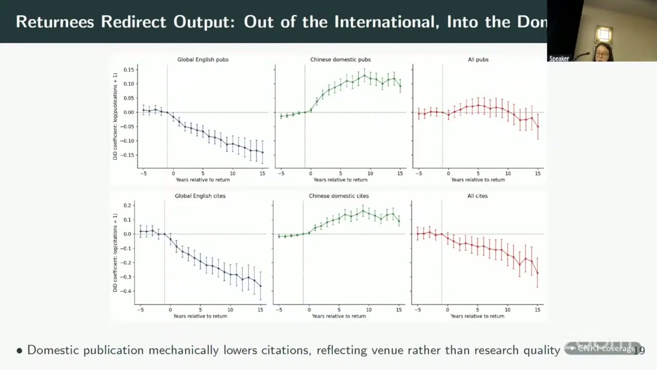
Six event-study panels, matched returnee-versus-stayer difference-in-differences, years −5 to 15 relative to return. Top row is log publications: Global English falls steadily to about −0.14 by year 15; Chinese domestic rises to about +0.12 by years 9 to 10; All pubs hovers near zero and dips at year 15. Bottom row is log citations: English falls to about −0.35; domestic rises to about +0.15; All cites drifts down to about −0.27. Footnote: domestic publication mechanically lowers citations, reflecting venue rather than research quality. — Slide at 04:15:34: “the returnees actually redirect output from the international journals into domestic journals. However, their total publication almost remains unchanged.”

The first result is a change of venue. English-language publications fall steadily against the matched stayers, Chinese-language ones rise, and the total barely moves. “If anything, there’s even a bit higher,” she said (04:15:38). Citations fall, especially English ones, and the slide’s footnote puts this down to venue rather than quality: a Chinese journal in the 1950s had fewer readers. That is a claim, and the next slide is the evidence offered for it.

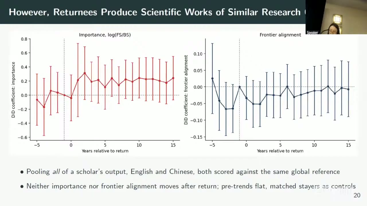
Two event-study panels, years −5 to 15 relative to return. Left, in red, “Importance, log(FS/BS)”: post-return coefficients all positive, mostly between 0.1 and 0.3, with wide intervals that all include zero. Right, in dark blue, “Frontier alignment”: coefficients between about −0.05 and 0 after return, intervals including zero, with dips to about −0.065 at years −3 and −2. Bullets: output pooled across English and Chinese and scored against the same global reference; neither importance nor frontier alignment moves after return. — Slide at 04:16:07: “We pull all of the scholar’s output in that year, both in English and Chinese, and score against the same global reference, and neither of these move after their return.”

Pool all of a scholar’s output, score it against a single global reference, and neither importance nor frontier alignment moves after the return. This is the result she leaned on, and it deserves one qualification. In the importance panel every post-return point is positive, around 0.1 to 0.3, and every interval includes zero (the slide does not state the confidence level). A questioner asked whether 0.2 meant 20% (04:17:31). She answered that the outcome is “the raw important score, not like the log of important score” (04:18:12), and conceded that the slide should state the economic magnitude (04:18:33). But the panel is labelled log(fs/bs), and the score is itself defined as a log ratio of forward to backward similarity. So 0.2 is about 0.2 log points of that ratio, roughly 22% (my arithmetic). “No detectable change” fits the intervals. “No change” says more than the chart does, and if the point estimates mean anything, returnees’ work became more important relative to the stayers’, which is an odd thing to undersell. The frontier-alignment panel also dips before the return, which the “pre-trends flat” bullet passes over.

What changed was direction. Her example is Qian Xuesen, whose name the captions mangle. At Caltech he worked on aerodynamics and propulsion, and in China on cybernetics and systems science. The field label stayed the same and the questions changed (04:18:38). Across all returnees, an llm rating of each scientist’s own papers before and after the return says that returnees changed their agenda more than stayers did and moved further toward applied work (04:19:04). Text-matched against the twelve priority areas of the 1956–67 12-Year Science and Technology Development Plan, their output lines up with what the state asked for (04:19:16). So the state told you what to work on, you worked on it, and on the paper’s yardsticks the work did not get worse.

Two questions from the floor went to the control group. The first questioner (the presenter seems to call on a “Santiago”) raised sutva: if my colleague leaves, I face less competition for journal slots, so the stayers are not a clean control (04:16:26). Her first answer, that isolated China meant little contact with the stayers (04:17:07), is about contact, not competition; on a second pass she said “Ah… I see” and promised the raw trends (04:17:24). If the effect is real it flatters the stayers and pushes every returnee-minus-stayer gap down, including the importance gap. The second questioner asked why I go home and my cohort-mate does not; perhaps I wanted to change topics (04:19:44). She pointed to the exit ban; the reply was that the ban gives variation over time, but within a cohort the choice to return is still selected, for instance by people who were not succeeding in us journals (04:20:28; the captions’ “ride based selection” is probably Roy-based). This goes to the heart of the direction result. In a matched DiD, “going home makes you change topics” and “people who want to change topics go home” produce the same picture. The classified list is the answer to both questions, and it is still pending.

What the returnees did for their colleagues

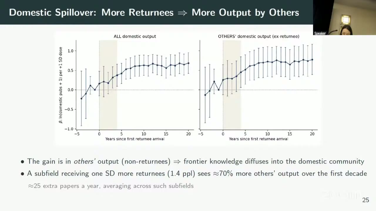
Two stacked event-study panels, years −5 to 20 since a subfield’s first returnee arrival, coefficient on log(domestic pubs + 1) per +1 SD returnee dose, with the first five post-arrival years shaded. Left, all domestic output, rising to about 0.6–0.7 from year 8. Right, others’ (non-returnee) output, rising to about 0.7–0.78. Early intervals are wide. Bullets: the gain is in others’ output, so frontier knowledge diffuses into the domestic community; one SD more returnees (1.4 people) gives about 70% more others’ output over the first decade, about 25 extra papers a year. — Slide at 04:23:04: “a sub field receiving one standard deviation more returnees sees actually 70% more of the non-returnee output over the first decade, which is about 25 extra papers a year”

The second design moves to cnki subfields. Each returnee is assigned to a modal subfield, the event is the first returnee’s arrival, and the dose is the standardized number of returnees. Each arrival cohort is compared with subfields that never got one, in a stacked event study (04:22:33). Domestic output rises with the dose, and the rise is in other people’s papers, not the returnees’ own. Per the slide, one more standard deviation of returnees (1.4 people) means about 70% more output by others over the first decade, about 25 extra papers a year. The intervals in the first five years are wide enough to hold almost anything, and the slides do not say how log-point coefficients become the percentages.

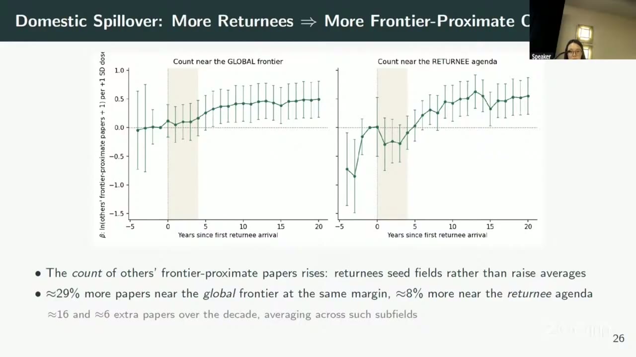
Two stacked event-study panels, years −5 to 20 since first returnee arrival, coefficient on log(others’ frontier-proximate papers + 1) per +1 SD dose. Left, count near the global frontier, rising to about 0.4–0.5 from year 5. Right, count near the returnee agenda: about −0.7 and −0.85 at years −4 and −3, below zero for most of the first five post-arrival years, then rising to about 0.4–0.6 from year 9. Bullets: about 29% more papers near the global frontier and about 8% more near the returnee agenda; about 16 and 6 extra papers over the decade. — Slide at 04:24:20: “≈29% more papers near the global frontier at the same margin, ≈8% more near the returnee agenda”; and at 04:23:50: “you will see there is a weird pretrend here”

The same design applied to frontier-proximate papers by others gives about 29% more near the global frontier and about 8% more near the returnees’ own agenda: about 16 and 6 extra papers over the decade. The returnee-agenda panel has a large pre-trend, about −0.7 and −0.85 four and three years before arrival. She called it “a weird pretrend” and said it comes from the returnees themselves shifting their agenda (04:23:50): the reference point moved, so local papers from before the arrival look far from it. The 8% is a first-decade figure, and the panel spends most of the first half of that decade below zero. A questioner suggested the treated fields might already have been better. She said summary statistics would help and argued that, since output near the global frontier rose after arrival, the returnees must have had better skills than the locally trained (04:24:30).

The channel is still descriptive. Of the returnees, 58% took university posts and 26% held leadership posts, and 17 of the 23 “Two Bombs, One Satellite” honourees were returnees (04:25:32). Asked whether the spillover runs through colleagues or students, she said that split is planned and not yet done (04:25:02).

Pricing the move

Schematic drawn for this note from the slides at 04:26:34 and 04:27:25, not the authors’ exhibit. Two country blocks of the stacked citation network plus a world-frontier sink. A returnee moves output share s_f from US field f to China field f, and each country keeps a share x of the field’s spillovers at home and leaks the rest to the frontier, which neither country’s value credits, so net world = gain − loss leaves it out. Arrow widths are not to scale, and how x enters the stacked network is not shown on any slide. Open the figure in a new tab

The last section turns all this into a number. The framework is adapted from Liu and Ma (2026) and a second paper whose citation is cut off on the slide (another slide cites Chen, Liu and Ma, 2026). The idea is that a scientist matters “not only because of his papers … but also because what is built upon it” (04:26:45). A field’s social value is its own output plus the discounted chain of spillovers it sets off through the citation network (deck slide 30):

\gamma'=\frac{\rho}{\rho+\lambda}\,\beta'\left(I-\frac{\Omega}{1+\rho/\lambda}\right)^{-1}

Here $\gamma$ is the vector of field values, $\beta$ is each field’s global output share, $\Omega$ is the field-to-field citation network, $\rho$ is the discount rate and $\lambda$ the rate at which knowledge becomes obsolete. Central fields are worth far more than their output. The top fields “warrant four to 18 times the R&D of the lower rank ones” (04:29:03), and returnees went disproportionately into central fields (04:29:17). The network is then stacked by country and re-solved (deck slide 31):

\text{China gain}=\frac{\psi\lambda}{\rho^2}\,s_f\,\hat\gamma_{CN,f},\qquad \text{US loss}=\frac{\psi\lambda}{\rho^2}\,s_f\,\hat\gamma_{US,f},\qquad \text{net}_{\text{world}}=\text{gain}-\text{loss}

Here $s_f$ is the returnees’ output share in field $f$ , $\hat\gamma_{CN}$ and $\hat\gamma_{US}$ are field values re-solved on the country-stacked network, and $\psi$ is a scale. Look at what is the same on both sides. It is the same scientist, the same output share and the same prefactor. Within a field, the gain-to-loss ratio is just $\hat\gamma_{CN,f}/\hat\gamma_{US,f}$ . The scientist did not get worse when she went home, and the matched DiD says so too. The country around her had a different value, and the whole result lives in that difference.

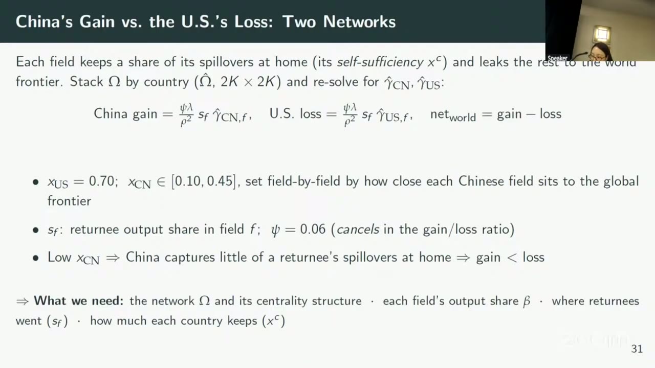
Slide titled “China’s Gain vs. the U.S.’s Loss: Two Networks”. Text: each field keeps a share of its spillovers at home (its self-sufficiency x^c) and leaks the rest to the world frontier; stack Omega by country and re-solve for the two country values. The China gain, US loss and net-world formulas follow. Bullets: x_US = 0.70; x_CN between 0.10 and 0.45, set field by field by how close each Chinese field sits to the global frontier; s_f is returnee output share and psi = 0.06 cancels in the gain/loss ratio; low x_CN means China captures little of a returnee’s spillovers at home, so gain is less than loss. — Slide at 04:27:25: “each field would keep a share of its spillovers at home, which we call the self-sufficiency rate, and leaks the rest to the [world] frontier”

What drives the difference, on the authors’ own reading, is the self-sufficiency share $x^c$ : the share of a field’s spillovers a country keeps at home. On the slide, $x_{US}=0.70$ and $x_{CN}$ runs from 0.10 to 0.45. The us number, she said, is computed “from domestic citation share” (04:27:43). The Chinese numbers are set field by field according to how close each Chinese subfield sits to the global frontier, “which is us” (04:27:56). Her intuition is a good one. In the us your colleagues can build on your papers, but in China “they don’t have very good peers to actually utilize their ideas. So the rest leaked to a frontier it could not yet use” (04:30:28). The limits should be stated plainly. The mapping from frontier proximity to $x_{CN}$ is not shown, how $x^c$ enters the stacked network is not shown, and the ratio is not decomposed across $x$ , $\Omega$ and $s_f$ . The headline therefore rests on calibrated home-retention shares. It is a calibration, not an estimate.

Two-panel slide headed “China’s Gain ≈ One-Third of the U.S.’s Loss ⇒ Net-World Loss”, with two unopened backup buttons, “Scarcity premium” and “China’s own network”. Left, a bar chart of per-returnee social value (ratio 34%): a green bar for China’s gain at +0.015, a red bar for the US loss at −0.045 and a grey bar for the global net at −0.030. Right, horizontal bars for the top returnee subfields (Materials Chemistry, Atomic and Molecular Physics, Electrical and Electronic, Aerospace Engineering, Mechanical Engineering and others), each with a short green China gain and a longer red US loss. — Slide at 04:30:43: “China’s gain offsets only a third of the US loss … the US loss is larger than Chinese gain everywhere, so the scientific value was actually destroyed, not just transferred”

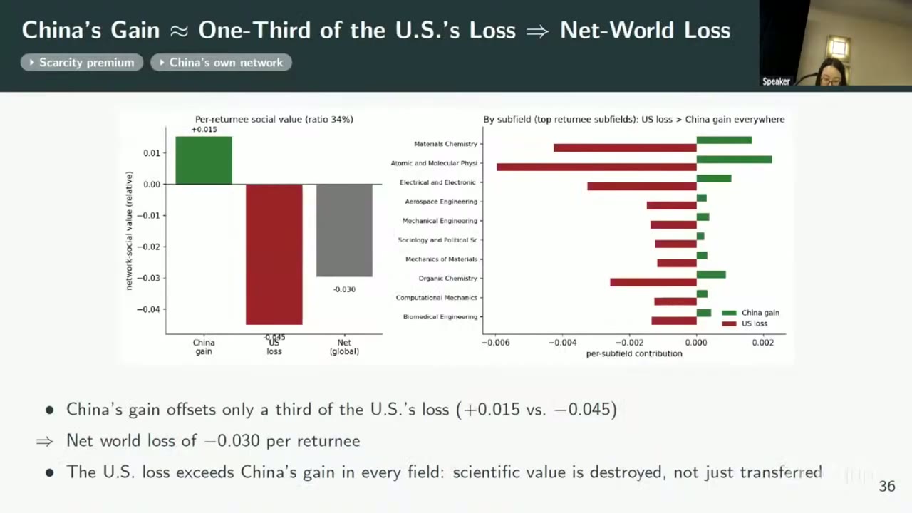
The output: per returnee, China gains +0.015 and the us loses −0.045, a ratio of 34%, for a net world loss of −0.030. The us loss is larger in every top returnee subfield. “The scientific value was actually destroyed, not just transferred” (04:30:53).

It helps to be precise about what “destroyed” means here, which is what the schematic is for. The net-world figure is gain minus loss: two home blocks. A spillover that leaks out of China to the world frontier is credited to neither country’s $\hat\gamma$ , so in this ledger it is gone. Whether it is gone in the world is a separate question. If the frontier “is us”, a reader will want to know who stands at the far end of that dashed arrow, and the slides do not say. (Two backup buttons, “Scarcity premium” and “China’s own network”, sat on the headline slide unopened. One of them may answer this.) The closing slide adds that subfields with more returnees became less reliant on us science, with a placebo of us reliance on China that stays flat (04:31:08).

What the room pushed on

The sharpest question came early (04:09:26). The famous returnees built missiles and atomic bombs, not journal articles. So is a publication outcome missing what they actually made? She agreed. Publications are the most measurable output of a planned economy with no patents, and much of the work was in secret national projects that cannot be measured, so the estimates are a lower bound (04:10:04). A follow-up, possibly from the chair, carried the point over to the welfare number (04:10:41): if China’s gain is counted in publications, it is probably understated. (The questioner said “one quarter”; the slides say a third.) Her answer: “totally … we take it” (04:11:09).

The last question asked whether a return today would still be a net global loss, now that China sits much closer to the frontier (04:32:44). She said China’s self-sufficiency has risen a lot since the 1950s and the network results “would be very different” (04:32:55).

Put those two answers together and the welfare section looks a little different. The ledger counts citations, so 17 of the 23 Two Bombs, One Satellite honourees enter it as people whose citations fell. And it prices the move at the absorptive capacity the returnees found when they arrived. The spillover section, meanwhile, shows them spending the next two decades raising that capacity. The calculation says the move destroyed value, and it gets there through a parameter the movers had been called home to change.