Optimal taxation, marriage, home production, and family labor supply

George-Levi Gayle and Andrew Shephard; published in Econometrica, January 2019, vol. 87 no. 1, pp. 291–326. PDF-only digest: no talk or discussant was found. Version used: the published version plus the online supplement.

Gayle and Shephard’s paper on taxing couples is, underneath, a paper about a price. The price is the wife’s Pareto weight, the $\lambda$ in every collective household model, which the literature has usually treated as a black box: a number that summarises “bargaining power” and that you estimate, condition on, and try not to think about too hard. Here it is not a black box. It is the price that clears the marriage market. If too many high-school men want to marry college women, the college women’s weight in those marriages rises until the queue clears, the same way a wage would. And once you have written down that the within-household split is a market-clearing price, a slightly alarming policy lever falls out: the tax you levy on single men changes how resources are divided inside marriages, because it changes what the men who marry are giving up.

The headline most readers will take away is a different one, about jointness. The optimal couples’ schedule in this model has negative jointness: the more your spouse earns, the lower your own marginal rate. That is the opposite of what the us does. It is also, by the paper’s own measure, not worth very much. Both points are worth walking through, but the price is the engine.

The model

There are two stages. In the second, after wages, taste shocks and children have been realised, a married couple is a Chiappori (1988, 1992) collective household: it maximises $(1-\lambda_{ij})$ times his utility plus $\lambda_{ij}$ times hers (eq. 2a in the paper, p. 296), each spouse choosing leisure, market hours and home hours from a discrete grid. Pooled earnings net of the tax $T(z_1, z_2)$ and fixed work costs buy a private good, which is split; home hours from both spouses produce a Cobb–Douglas home good $Q$, which is not split, because it is public (eq. 12, p. 303). That publicness is the economic gain from marriage. Singles solve the same problem alone.

In the first stage, a frictionless Choo and Siow (2006) marriage market clears. Each person sees an idiosyncratic Type-I extreme-value payoff $\theta$ attached to each spouse type (three education groups for each sex), compares the expected value of staying single with the expected value of marrying each type, and picks the best. That gives a logit demand from type-$i$ men for type-$j$ wives and a logit supply of type-$j$ women to type-$i$ men, and the nine weights are whatever makes them equal:

This is eq. 7 in the paper (p. 298): $\mu_{ij}$ is the measure of type-$i$ men married to type-$j$ women, $\mu^d_{ij}$ and $\mu^s_{ij}$ are men’s demand and women’s supply for that pairing, and $T$ is the tax system, so the vector of Pareto weights $\boldsymbol\lambda$ plays the role of the price vector.

The link between the stages is that $\lambda_{ij}$ determines the expected values that drive the first-stage choices, and the thing that makes the whole paper go is that utility is imperfectly transferable (following Galichon, Kominers, and Weber 2019). Under transferable utility the weight would just be a lump-sum transfer: it would move who gets what, but not how the couple spends its time, and taxes could not move the relative standing of spouses (p. 293). With a curved utility frontier, the market conditions that set $\lambda$ also change hours, and the tax schedule can reach inside the household. Chiappori, Costa Dias, and Meghir (2018) combine collective households and matching with transferable utility and, as the paper notes, do not ask optimal-tax questions; Kleven, Kreiner, and Saez (2009), the benchmark on taxing couples, take the married unit and its internal allocation as given.

The estimation is on the 2006 American Community Survey plus pooled American Time Use Survey data for home time, for singles and household heads aged 25 to 45, across nine Census divisions treated as separate marriage markets, each run under its actual 2006 federal and state tax-and-transfer rules. The identification of $\lambda$ is the nice part. Differences in sex ratios by education across divisions do not change the value of being single, so they move marriage choices only through the weights; the ratio of men’s to women’s responses then pins $\lambda_{ij}$ down (Proposition 2, p. 304, with the proof in the online supplement). That is the distribution-factor logic of Blundell, Chiappori, and Meghir (2005) and Browning, Chiappori, and Lewbel (2013), with the population vector cast as the distribution factor. The estimated weights “typically favor the husband” (p. 293), and they move the way a price should: a college-educated woman gets about 0.44 with a college-educated husband and about 0.61 with a high-school one (p. 307). The model also delivers a quietly striking line from the fit to the utility frontiers, which cover New England matches with a college-educated husband: “only in the joint ‘college and above’ matches does the expected value of marriage exceed that of singlehood. Heterogamous marriages are therefore primarily explained by the noneconomic gains” (p. 309). The payoff there is to a spouse type, not to a particular person, so it would be a stretch to call it love; it is whatever the economics does not explain.

The planner then takes the estimated primitives as fixed and, following the structural template of Blundell and Shephard (2012), chooses a piecewise-linear schedule for singles and a fully nonparametric one for couples (tax levels on a 10×10 grid of earnings nodes, triangulated in between, 65 parameters in all), with marriage-market clearing imposed as equality constraints so that the equilibrium is computed at the optimum rather than at every candidate (pp. 313–314). No primary- or secondary-earner distinction is imposed; “low, medium and high spousal earnings” are defined by earnings, not by sex. The objective is an individualistic welfare function that sums a transform of each man’s and each woman’s utility, single or married, with inequality aversion indexed by $\delta$. Two features matter. Because it counts spouses separately, inequality inside a household lowers social welfare (p. 299), so the planner’s view of a couple can differ from the couple’s own weights. And even at $\delta = 0$ there is “a considerable redistributive motive” (p. 317), because individual utility is concave.

Negative jointness

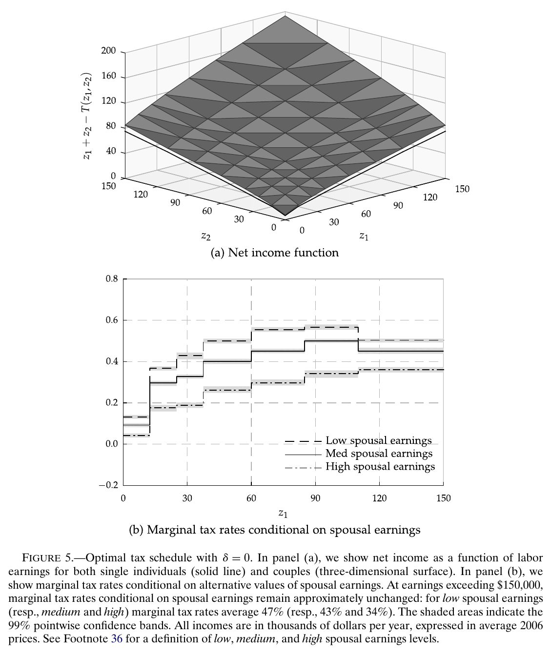
Figure 5 is the optimum at $\delta = 0$, and panel (b) has three features. Conditional on spousal earnings, your marginal rate rises with your own earnings and dips a little at the top, which is Mirrlees (1971) doing what Mirrlees does. Rates are close to zero at low earnings, which is Saez (2002): when the extensive margin is the elastic one, you do not want to tax the first dollars earned. And the three lines never cross, low spousal earnings on top and high at the bottom: above $150,000 of own earnings the rates average 47, 43 and 34 percent (Figure 5 caption). That is negative jointness. The shaded bands are 99 percent pointwise bands from 200 draws of the parameter estimates, so their thinness is about sampling error, not about whether you believe Type-I extreme-value marital payoffs.

The intuition is Kleven, Kreiner and Saez’s. Start from individual taxation. A transfer from a low–high couple to a low–low couple is worth more to a redistributive planner than an equal transfer from a high–low couple to a high–high couple costs, and it has no first-order revenue cost, so a little negative jointness raises welfare. Kleven, Kreiner and Saez derived this with a unitary household, and noted it would survive in a collective one if the planner respected the household’s weights. This planner does not, and the weights are equilibrium objects. The paper does not prove the result survives; it says, with some care, that “our quantitative analysis does suggest that the negative jointness property is somewhat more general” (p. 315). (Frankel (2014) showed that assortative mating attenuates negative jointness; consistent with that, the supplement’s perturbation that weakens assortative mating widens the gap between the lines, and makes individual taxation costlier.) At this optimum, married women’s employment is 87 percent against 79 percent in the estimated baseline, with hours among the employed about unchanged, and the overall marriage rate is 5 points higher (p. 317), all of it a model counterfactual.

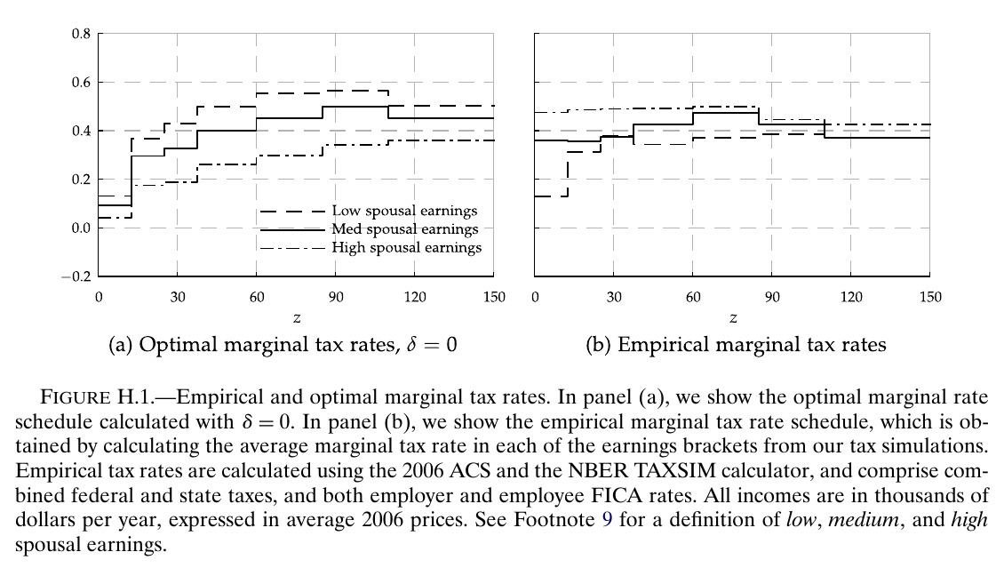
Figure H.1 in the supplement puts the optimum next to the 2006 us system, and the useful comparison is one line. The high-spousal-earnings line, the lowest at the optimum, is the highest in the us: aggregating a couple’s income under a progressive schedule is positive jointness, so the second earner in a high-earning couple starts on the upper steps. The other two lines do not neatly swap; in the us panel low and medium overlap and even cross. And do not compare levels across the panels. The us series are population averages by bracket and include federal and state taxes plus both halves of fica, whereas the optimal problem’s revenue target is income tax net of transfers. The ordering of the high line is the result; everything else in the panel is texture.

How much it is worth

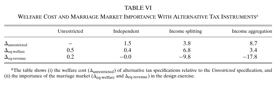
Now force the planner into one of three familiar boxes, each re-optimised within its form: individual taxation, joint taxation with income splitting, or joint taxation with income aggregation (the us-style one). The cost is measured through the dual, as the revenue lost while delivering the unrestricted schedule’s welfare, and it comes out at 1.5, 3.8 and 8.7 percent of tax revenue respectively (p. 318; the first row of Table VI). Two things follow. Individual taxation, the zero-jointness box, gets you nearly all the way there, which the authors concede directly: “the actual welfare gains from introducing this jointness (relative to a system of independent taxation) appear somewhat modest” (p. 318). And aggregation is the worst box by a distance. That 8.7 percent is the cost of the best aggregation schedule, not a score for the actual 2006 code, which is never scored. Under aggregation the marriage rate is also 15 points lower, with less assortative mating (supplement p. 14).

The lower two rows ask what the planner loses by ignoring the marriage market: design the schedule holding weights, pairings and payoff distributions fixed, then let the market clear and see how far off you are. For the unrestricted schedule and for individual taxation, not much, about half a percent of revenue as a lower bound. For the two joint schemes, 6.8 and 3.4 percent, plus large revenue misses (p. 322). This is a tidy result that deserves more attention than the jointness headline. The schedules that treat marriage non-neutrally are exactly the ones whose design you get wrong if you take marriage as given, which is a decent argument for not treating marriage non-neutrally.

The surprising part: taxing single men

Here is where the price earns its keep. Proposition 5 decomposes the welfare effect of nudging any tax parameter $\tau$ at $\delta = 0$:

This is eq. 14 in the paper (p. 319): $U^i_{i0}$ and $U^j_{0j}$ are the expected values of single men and women, $U^i_{ij}$ and $U^j_{ij}$ those of a type-$i$ husband and type-$j$ wife, the $\mu$’s weight each group by its size, and the last term, which exists only because the planner and the household weigh spouses differently, is nonzero whenever $\lambda_{ij} \neq 1/2$.

Since the husband’s value falls as his wife’s weight rises, that last term is positive whenever a reform raises the weight of a wife who is under-weighted. Changes in who marries whom have no first-order effect; the envelope theorem takes care of them. So consider, as the paper does, a small tax increase on single men. Their outside option falls; at the old weights more men now want to marry than women will accept; the wife’s weight must rise to clear the market; within-household inequality falls, “offering a potential welfare gain” (p. 319). Potential, because the reform still has its ordinary mechanical and behavioural effects on the single men you just taxed, and those go in the first line of the equation. But the channel is real, and it is odd: the schedule for people who are not married is a lever on how marriages divide their resources.

Let taxes depend on gender and the planner uses it. Married women’s marginal rates end up about 5 points below their husbands’, single women’s 5 to 10 points below single men’s, the wife’s Pareto weight rises in every pairing, and the welfare gain is 5.6 percent of revenue over the best gender-neutral schedule (p. 320). Most of that runs through singles’ taxes: gender the couples’ schedule alone and the changes are “much smaller” (fn. 39, p. 320). Alesina, Ichino, and Karabarbounis (2011) conjectured that taxes could move within-household inequality; this is a structural model in which they do, entirely through the marriage market. The same channel is why a larger gender wage gap raises the value of jointness: cut every female type’s mean log-wage offer by 0.5 and the gain of the unrestricted schedule over individual taxation becomes almost 4 percent of revenue, rising to around 6.5 percent for a cut of 1.0 (p. 322; supplement pp. 16–17), with singles’ rates up about 10 points to prop up wives’ weights. Those are imposed shocks, not history.

Objections the paper itself anticipates (no discussant was found; this note stands in for one)

Marriage is static and irrevocable, with no divorce, life cycle or cohabitation, although cohabitants are about 7 percent of the sample’s households and are an obvious place for tax avoidance to go (fn. 10, p. 295; p. 323). Wages do not respond to taxes. The Type-I extreme-value marital payoff, which the authors single out as their strongest assumption, carries existence, identification, computation and the welfare decomposition (p. 304). The planner’s inequality aversion is a choice, and gender tagging raises horizontal-equity concerns the paper flags itself (fn. 39, p. 320). And negative jointness is a quantitative finding under these weights, not a theorem.

What you are left with is a paper whose loudest result, that the us has jointness backwards, comes with the authors’ own note that getting it right is worth a percent and a half of revenue, and whose quietest result is that one of the better ways to help married women in the model is to raise taxes on the men who are not married to anyone.

References