Displacement Risk and Asset Returns

Nicolae Gârleanu, Leonid Kogan and Stavros Panageas, Journal of Financial Economics 105(3), 491–510 (2012). Digested from the authors’ final manuscript plus the extended (internet) appendix; no talk video was found, so this note is pdf-only.

Gârleanu, Kogan and Panageas start from an observation that every incumbent already knows: innovation is good news for the economy and bad news for whoever was doing well under the old technology. A new variety raises output and takes market share from the varieties that already exist; a new technology raises average wages and devalues skills trained on the old one. None of that is a puzzle: aggregate consumption goes up, and the representative agent is happy.

The paper’s point is that there is no representative agent to be happy, because the people who capture the gains from innovation are, for the most part, not yet born. You are alive today, you own today’s firms and today’s human capital, and you would very much like to insure against the arrival of a cohort of inventors who will make both less valuable. You have a complete set of Arrow–Debreu securities. You can buy any state-contingent claim you like from anyone else who is alive. What you cannot do is sell the downside of an innovation boom to the inventors who will profit from it, because they are not around to take the other side. The market is complete among the living and missing exactly one counterparty, the future.

So the paper’s recategorization is this: innovation risk is aggregate good news that is a priced bad state, because the stochastic discount factor that matters belongs to the current population, not to aggregate consumption. The authors call the resulting factor “displacement risk”, and they use it to explain three things at once: the value premium, an equity premium larger than aggregate consumption risk can justify, and a riskless rate lower than it would suggest. The value premium is the most interesting of the three, because in this model growth stocks are the one asset you can buy that pays off when the future arrives and displaces you. They are insurance, and the value premium is what that insurance costs.

The model: complete markets with a missing generation

The demographics are Blanchard (1985) perpetual youth. Each year a mass $\lambda$ of agents dies and a mass $\lambda$ is born, so the population stays at one. Newborns are either entrepreneurs (share $\phi$) or workers (share $1-\phi$). Preferences are crra with an Abel (1990)-style “keeping up with the Joneses” term, weight $\psi$ on own consumption and $1-\psi$ on consumption relative to the aggregate. The authors say plainly that the Joneses term “only helps at the calibration stage”, by pushing the interest rate down; it is not what drives the mechanism.

Production is Romer (1990) expanding variety, with the growth made exogenous. A competitive final-good firm combines labour with a continuum of $A_t$ intermediate goods, each made by a monopolist that owns its blueprint forever. The blueprint stock grows by a Gamma-distributed shock, $\log A_{t+1}=\log A_t+u_{t+1}$, and $u$ is the innovation shock that does all the interesting work. There is a separate log-random-walk tfp shock $\varepsilon$, which turns out to play a minor role. Weights in the production function tilt demand towards newer varieties at a rate set by $\chi$.

Proposition 1 then gives closed forms, and the key one is the profit of a single blueprint, $\pi^I_{j,t}=(1+\chi)(j/A_t)^{\chi}\alpha(1-\alpha)Y_t/A_t$ (eq. 20). Output rises with $A_t$ as $A_t^{1-\alpha}$, but each existing blueprint’s profit is divided by $A_t$ and then penalised again through the vintage term. So when $u$ is large, the economy gets richer and every existing firm gets a smaller slice of it. That is profit displacement. (The text around Prop. 1 calls intermediate profits “identical for all $j$”, which eq. 20 contradicts whenever $\chi>0$; follow the equation.) Aggregate profits stay a constant $\alpha(1-\alpha)$ share of output, and that is the useful distinction the paper draws: dividends of all firms alive at each date are cointegrated with consumption, while dividends of a fixed set of firms, the ones you can actually own today, are not.

Workers get the same treatment. A worker’s efficiency units decay with innovation, $\log q_{t+1,s}=\log q_{t,s}-\rho u_{t+1}$, while newborns arrive with an endowment that rises with the shock in their year of birth, so aggregate efficiency stays constant. A big innovation year makes the young more productive relative to the old.

Then comes the allocation of the new blueprints’ value, which is where the model decides who gets paid. A fraction $\kappa$ goes to arriving entrepreneurs, split between new value firms ($\eta\kappa$) and new growth firms ($(1-\eta)\kappa$). The remaining $1-\kappa$ goes to existing growth firms, with the cohort of growth firms born at $s$ collectively receiving $(1-\kappa)\frac{1-\varpi}{\varpi}\varpi^{t-s}$ (eq. 12), shared equally within the cohort. Value firms never get new blueprints. Growth firms get fewer as they age, so today’s growth firm is tomorrow’s value firm, and any fixed set of firms shrinks towards zero market share. These are shares of the value of new blueprints, not counts, and they are assumptions rather than outcomes of anyone’s R&D decision. With $\kappa=0.9$ in the calibration, 90% of the rents from innovation go to people who were not alive to trade beforehand.

Here is the wedge in one equation. Living agents share risk perfectly with each other (their consumption is perfectly correlated, fn. 13), so the sdf is the marginal utility growth of any survivor. But survivors’ consumption growth is aggregate consumption growth minus whatever newborns take:

This is eq. 24 in the paper: $\xi$ is the sdf of the living, $Y$ is output (equal to aggregate consumption), $\beta$, $\gamma$ and $\psi$ are the discount factor, risk aversion and own-consumption weight, $\lambda$ is the birth rate, and $\phi^i c^i_{t+1,t+1}/Y_{t+1}$ is the consumption share of newborn workers and entrepreneurs, so the bracket, which the paper writes $(1-\lambda)^{-1}\upsilon(u_{t+1})$ and calls the displacement factor, is the adjustment that turns aggregate growth into survivors’ growth.

The bracket falls in $u$ (eq. 25): big innovation years hand a bigger slice of tomorrow’s output to the arrivals. This is intergenerational incompleteness, not idiosyncratic incompleteness, and the authors are careful to separate themselves from Constantinides–Duffie (1996) and Heaton–Lucas (1996). They also say what a test should look for: “imperfect inter-generational risk sharing instead of imperfect risk sharing among existing agents.” Eq. 24 survives bequests, government debt and transfers, and adjustable capital, which only rescale the factor. It does not survive a representative altruistic dynasty, which sets the normalised factor to one and switches the whole mechanism off (fn. 14). Let parents internalise their unborn children’s gains and the counterparty is no longer missing.

A premium with no aggregate risk, in the limit

Lemma 1 is the cleanest statement of the idea, and it is a limit result, so read it as one. Shut down tfp risk ($\sigma=0$), let $\rho>0$, give all new blueprint value to newborns ($\kappa=1$), impose two parameter inequalities, and send $\alpha\to1$. Then the variance of output growth goes to zero, but the sdf still rises in $u$, and stocks earn a positive premium. Innovation in that limit is pure redistribution from old firms and old workers to new ones, and pure redistribution is enough to price risk when the losers can’t trade with the winners. The authors themselves note that profits vanish at $\alpha=1$, so the limit is “of limited practical relevance”. It is an existence proof for the mechanism, not a calibration.

Growth stocks as insurance

Every stock in the model is a time-$t$-known mix of two things: assets in place, which earn a share of a shrinking pie, and the option to receive future blueprints.

This is eq. 33 in the paper (with the signs from eq. 34): $R^a$ is the return on assets in place, $R^o$ the return on pure growth opportunities, and $w^o_t$ the growth-option weight, zero for value firms and between zero and one for growth firms.

Growth options pay off exactly when the living are displaced. So, given that the sdf rises in $u$, they hedge displacement, and value firms, which are all assets in place, carry the full exposure. The paper’s sign argument leans on Lemma 1’s limit; in the calibration the sign is confirmed numerically, with $E(R^a-R^o)=0.102$ at $\gamma=10$. A nice by-product: $\log R^a-\log R^o$ does not depend on $\varepsilon$ and falls in $u$, so the value-minus-growth return is a mimicking portfolio for the unobservable displacement factor. That is a structural reason for hml to show up as a factor, rather than just a reason for value to earn more on average.

The same logic delivers the other two results. Incumbents’ dividends are not cointegrated with consumption, so they can be volatile, and they load on a priced shock, so the equity premium is high. Survivors’ consumption grows more slowly and more riskily than the aggregate, so the riskless rate is low. What the model does not have is any time variation in the riskless rate, conditional premia or volatility. It is a model of unconditional moments.

Finding displacement in cohorts

You can’t observe $\upsilon(u)$ directly, but the model tells you where it leaves fingerprints: in the consumption of successive cohorts. If a big innovation year makes newborns richer relative to survivors, the cohort born that year should consume more for the rest of its life. Write household log consumption as a cohort effect plus a time effect, and Lemma 3 links the cohort effects to the displacement factor:

These are eqs. 35 and 39 in the paper: $a_s$ is the cohort effect, $b_t$ the time effect, $u$ the innovation shock, $\upsilon/(1-\lambda)$ the displacement factor, and $z_{s+T}-z_s$ a stationary difference, so the permanent component of cohort-effect increments is minus the log displacement factor. (Eq. 35 prints the residual’s subscript as $t$, while eq. 38 defines it with $s$.)

Mind the minus sign, because the paper’s own prose occasionally drops it. New cohorts doing well is the same event as survivors being displaced. So the prediction is that cohort increments covary positively with growth-minus-value returns.

The extended appendix makes a more general claim, and it is worth stating its conditions. In any overlapping-generations economy with a crra Euler equation among the living and a stationary newborn consumption share, the permanent part of the log sdf splits into a “rising tide component” from output and an “intergenerational distribution” component from cohort effects. That is independent of the displacement story. It is not independent of preferences: the appendix suppresses the Joneses term, and with the paper’s own $\psi<1$ the output coefficient is $-1+\psi(1-\gamma)$ rather than $-\gamma$. It tolerates Euler-equation wedges only if they wash out in the long run, which is why the authors frame the results as about “long-run returns”.

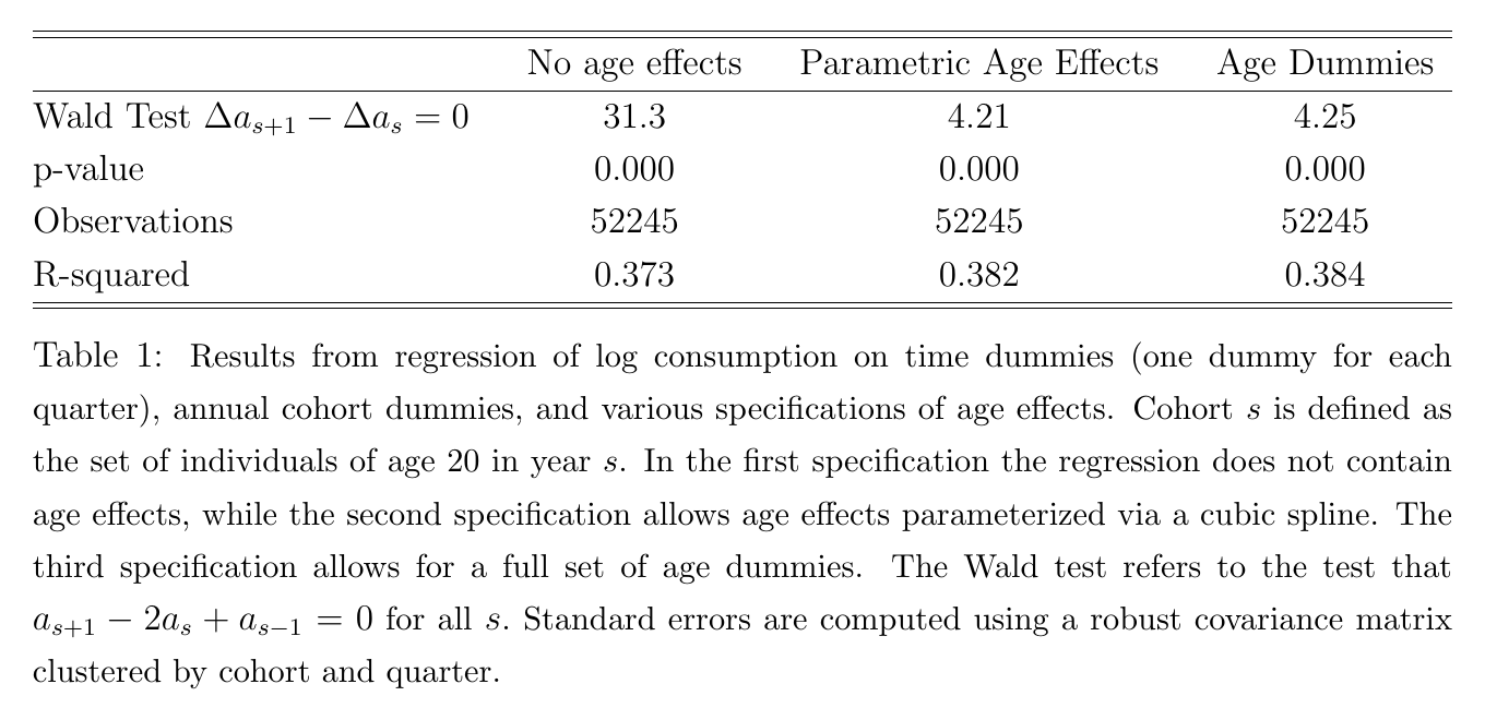
The data are the Consumer Expenditure Survey: household log expenditure on quarterly time dummies, annual cohort dummies and log household size, with a cohort defined as households aged 20 in year $s$. With age, time and cohort together, only second differences of cohort effects are identified (first differences up to a constant, which leaves their standard deviation alone). Table 1 asks whether all second differences are zero: the Wald statistics are 31.3 with no age controls, 4.21 with a cubic age spline and 4.25 with full age dummies, on 52,245 observations, all with printed p-values of 0.000 (rounded, not literally zero). Cohort effects exist. That is the necessary first step and not much more.

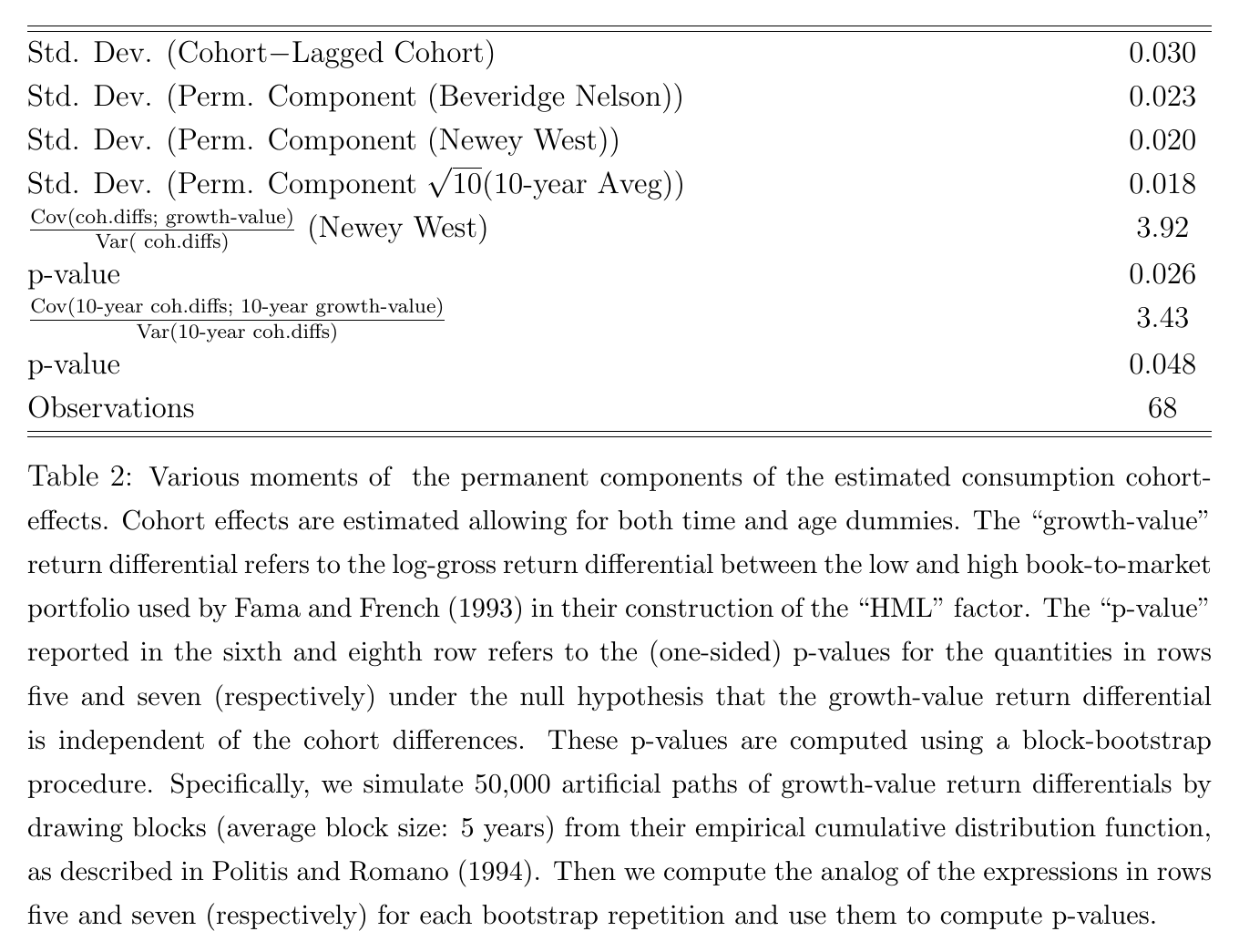
Table 2 does the work. The cohort increments have a standard deviation of 0.030, and the permanent component, by three different estimators, between 0.018 and 0.023. That is a displacement factor with roughly 2% annual volatility, not far below the 3.3% volatility of aggregate consumption growth. The covariance of cohort increments with the growth-minus-value log return, divided by the variance of the increments, is 3.92 (one-sided bootstrap p = 0.026), and 3.43 (p = 0.048) with ten-year differences. The sample is 68 cohort increments, cohorts 1927 to 1995, with the smallest cohort at 199 households and the median at 657. The bootstrap is 50,000 block paths, and blocks of one to ten years all give p below 5%. “Growth-minus-value” here is the low-minus-high book-to-market portfolios behind hml, in log gross returns.

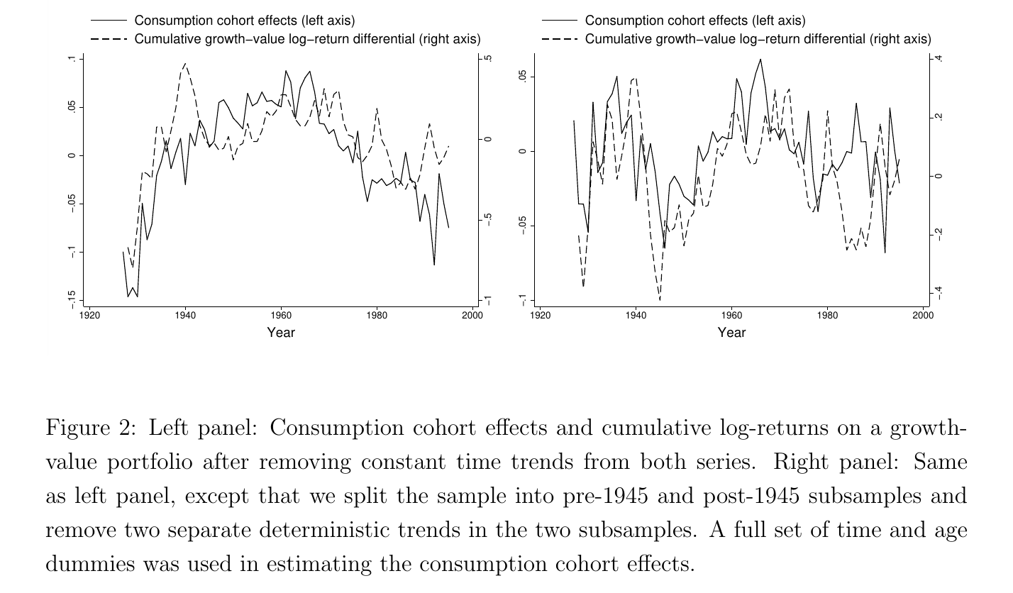
Figure 2 overlays detrended cohort effects on the cumulative growth-minus-value return. They move together at low frequency, and the right panel, with separate trends before and after 1945, looks cleaner than the left. It is a picture, not a test.

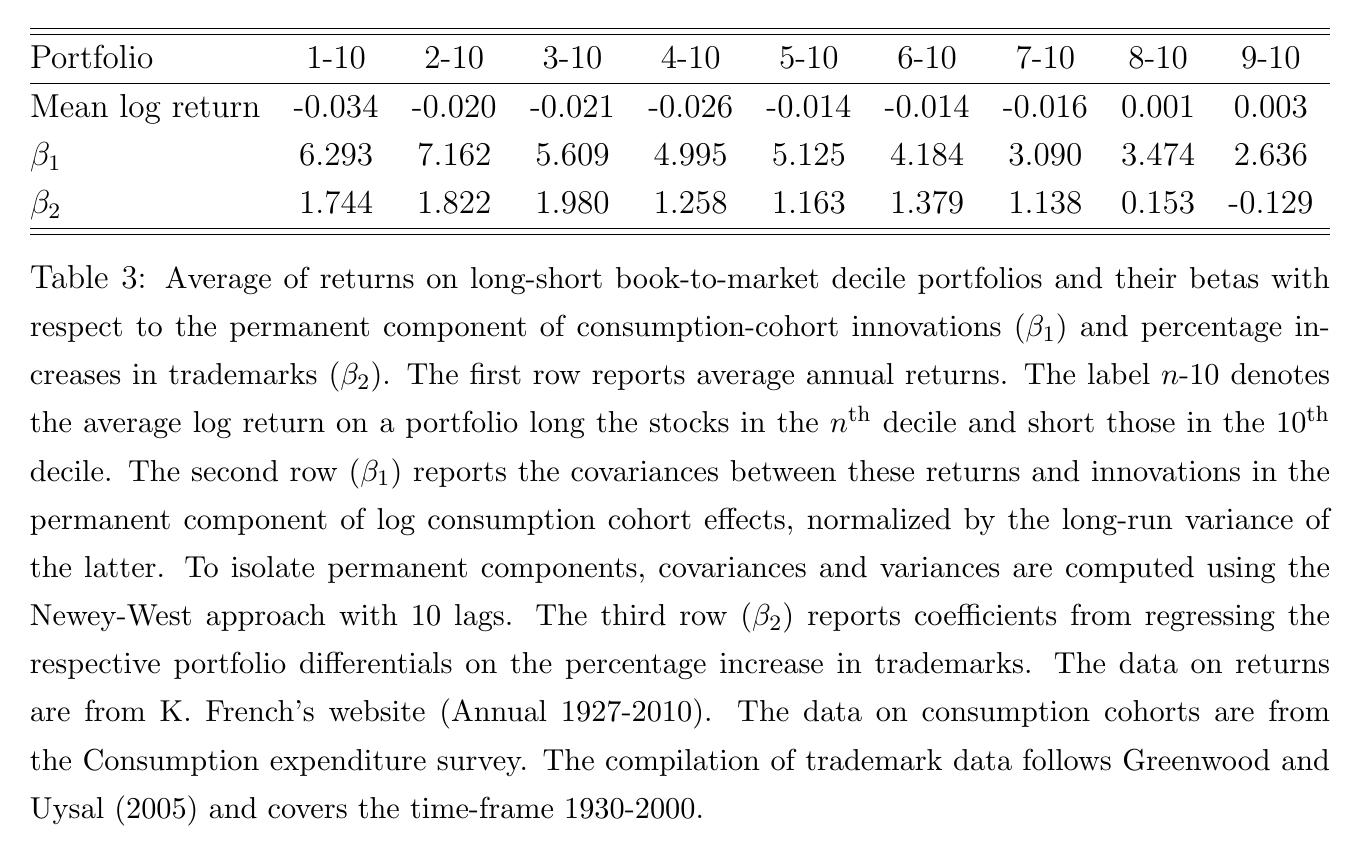
Table 3 pushes into the cross-section of book-to-market deciles, each against decile 10. The lowest decile spread earns −0.034 a year with a beta of 6.293 on permanent cohort innovations and 1.744 on trademark growth; the 9−10 spread earns 0.003 with betas of 2.636 and −0.129. The direction is right. The decline is not monotone (the cohort beta peaks at 2−10, and 8−10 exceeds 7−10), and no standard errors are reported.

The calibration, and the one surprising thing

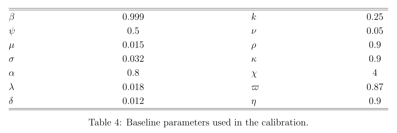
Table 4 sets $\alpha=0.8$, so the profit share $\alpha(1-\alpha)$ is 16% against 15 to 18% in the national accounts. It sets $\lambda=0.018$ (the prose says 0.02; the table is the one to use), $\psi=0.5$ to get the interest rate down, and $\kappa=0.9$, $\varpi=0.87$, $\eta=0.9$. The innovation parameters are chosen jointly to hit cohort-effect volatility and dividend moments, and $\kappa$ and $\varpi$ to hit aggregate E/P and the cohort covariance ratio. That last one matters later: the 3.92 from Table 2 is a calibration target, not an out-of-sample check. Risk aversion $\gamma$ is left free, at 10, 12 or 15. The share $\phi$ of entrepreneurs among newborns is not reported anywhere.

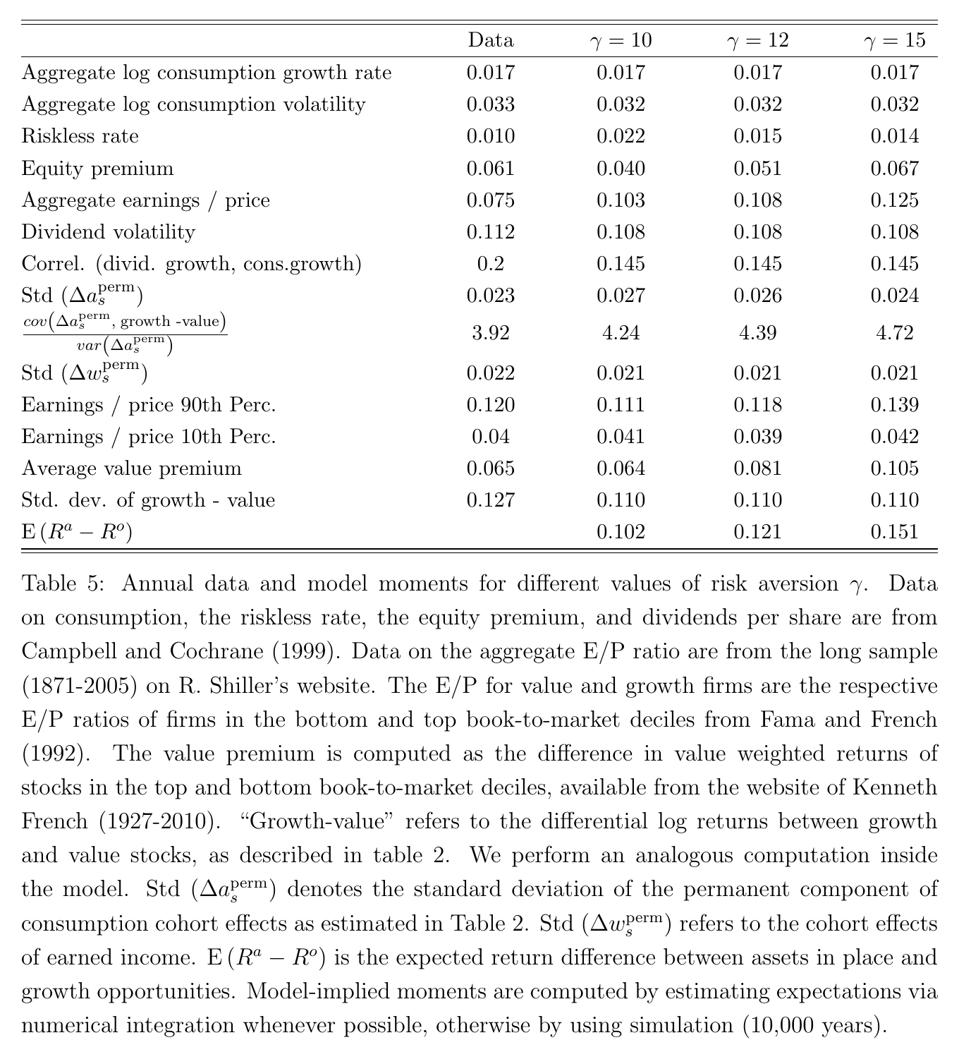
At $\gamma=10$, Table 5 gives a value premium of 0.064 against 0.065 in the data and an equity premium of 0.040 against 0.061. The authors read the latter as about right, citing Barro (2006): the model has no leverage, so an unlevered premium should be about two-thirds of the observed one. They concede that the model needs “relatively high levels of risk aversion”. The misses are honest ones: the riskless rate is 0.022 against 0.010, aggregate E/P is 0.103 against 0.075, and to match the equity premium you need $\gamma=15$, at which point the value premium overshoots to 0.105. The targeted moments overshoot too, 4.24 against 3.92 for the covariance ratio and 0.027 against 0.023 for the permanent cohort volatility.

Now the surprising part, which is in Section 5.3 and is easy to read past. You might think this model gets its equity premium by making survivors’ consumption much riskier than aggregate consumption. It doesn’t. Once the model is disciplined by the cohort data, survivors’ consumption-growth volatility is 0.039, against 0.032 for the aggregate. That is barely more risk. The premium comes from the other side of the covariance: incumbents’ dividends. Because they are not cointegrated with consumption, they can be volatile, about 0.10 in the paper’s back-of-the-envelope $\sqrt{0.032^2+0.095^2}$, and almost all of that volatility loads on $u$. The log sdf has an $\varepsilon$ term with standard deviation 0.18 and a $u$ term with standard deviation 0.24 (eq. 41). Treat everything as Gaussian and the premium is $0.18\times0.032+0.24\times0.095=0.029$; the remaining gap to 0.04 comes, the authors say, from the skewness of the Gamma shock. (Table 5 reports model dividend volatility of 0.108, not 0.10, and the paper does not reconcile the two numbers.)

So the trick is that the priced shock looks like good news in every aggregate series you would normally check. gdp up, consumption up, wages up, and your portfolio down. A consumption-capm econometrician who looks for a bad state in aggregate consumption will not find one, because it is not there. It is in the distribution of consumption across generations.

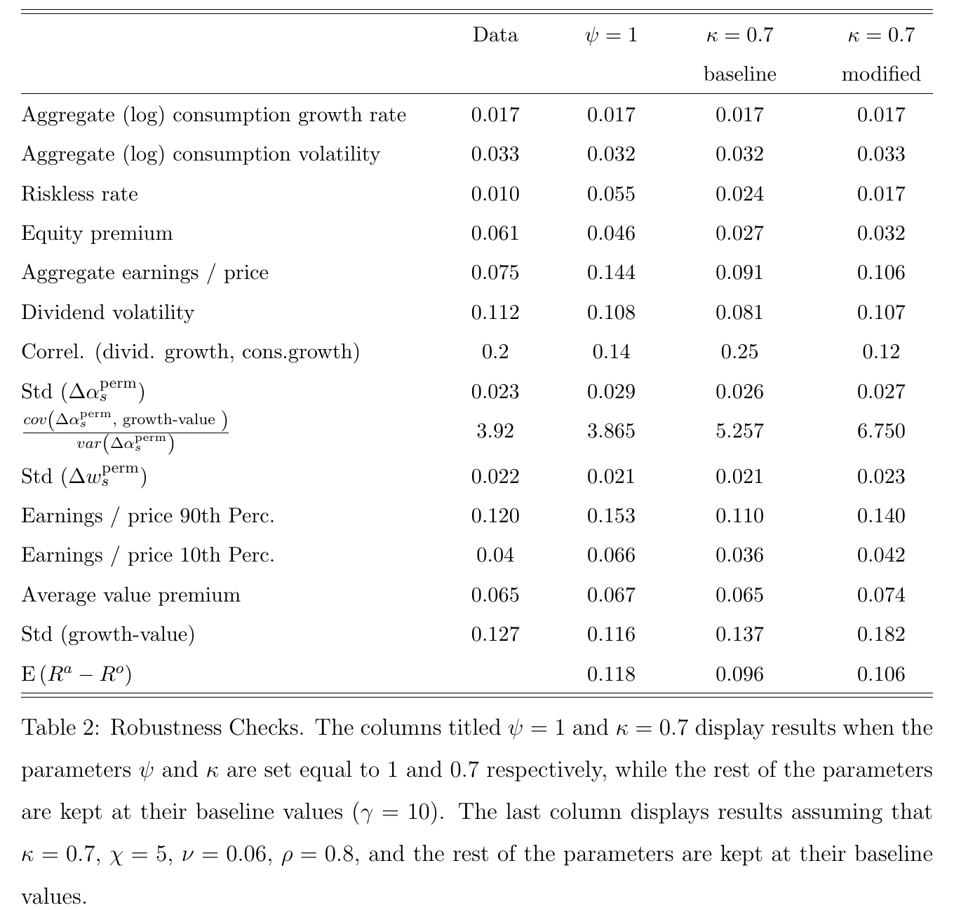
The extended appendix’s robustness table is worth reading against the main text. Under crra ($\psi=1$) the riskless rate is 0.055 (the main text says 5.7%) and aggregate E/P is 0.144, which the main text’s “slightly improved along all dimensions” does not quite cover; the appendix itself concedes that the riskless rate and all E/P ratios rise. Lowering $\kappa$ to 0.7 is the more informative experiment. The value premium holds at 0.065, but the equity premium falls to 0.027. A partial refit (with $\chi=5$, $\nu=0.06$, $\rho=0.8$) brings the equity premium to 0.032 and the value premium to 0.074, at the cost of a covariance ratio of 6.75 and a growth-minus-value volatility of 0.182, both well above their data targets. The authors defend $\kappa=0.9$ as the share of human capital and labour in innovation, which in Romer is close to one.

Weak points, our own reading (no discussant exists)

The rent split does a lot of the work and is assumed. $\kappa$, $\eta$ and $\varpi$ decide who captures innovation rents, and the equity premium is sensitive to $\kappa$ while the value premium is not. The paper’s answer, that endogenising innovation “would add complexity without altering the intuitions or the results”, is plausible for the intuitions and untested for the numbers.

The identification is thin. Sixty-eight cohort increments, one-sided p-values of 0.026 and 0.048, and early cohorts inferred from old households observed in the cex, so selection and survivorship could load on cohort. And the general decomposition cuts both ways. If the permanent cohort component prices long-run returns whatever drives it, then a priced cohort factor need not be innovation. Depression and war cohorts, education and fiscal transfers would all show up in $a_s$ (the paper argues transfers only rescale the factor), and the only innovation proxy offered is the trademark beta in Table 3, which has no standard errors.

The fit is not out of sample. The covariance ratio and the cohort volatility are targets, and the model overshoots both. Risk aversion of 10 to 15, Joneses preferences needed to keep the riskless rate below 5.5%, and no time variation in anything mean the model says nothing about return predictability, which is where much of the action on value has been.

Smaller things: growth versus value is a stylised binary with deterministic ageing (the authors call that “relatively easy to overcome”), displacement works through quantities with a constant mark-up, and the three tables measure “value minus growth” three different ways, decile spreads in Table 3, hml portfolios in Table 2 and a value-weighted top-minus-bottom decile in Table 5, so their magnitudes are not interchangeable. (Table 5’s note also labels the value and growth E/P deciles the opposite way from convention.)

None of this takes away the main idea, which is clean and still underused. Complete markets are complete among the people present, and the people who will capture the next technology are not present. So the economy has a factor that every aggregate series reads as a boom, every incumbent experiences as a loss, and the only hedge sold to incumbents is a ticket on the firms most likely to be in on the next thing. The price of that ticket is a lower expected return, which is a fairly polite way of saying that growth stocks are bought by people who are afraid of the young.

References