Technological Growth and Asset Pricing

Nicolae Gârleanu, Stavros Panageas and Jianfeng Yu, Journal of Finance 67(4) (2012), pp. 1265–1292. Published version, with its Internet Appendix; no recorded talk.

Gârleanu, Panageas and Yu’s paper is about the gap between a technology being invented and a technology being used. That gap is the reason it sits in a collection on growth and asset pricing: invention here is pure luck, a Poisson arrival nobody chooses, and everything interesting happens in adoption. A breakthrough lands, and on the day it lands nothing is produced with it. The railroad, electricity or the Internet exists only as a set of options held by firms that have not yet paid to build the thing. Output rises only as those options are exercised, slowly and in a particular order. Meanwhile the stock market is full of the options, and options are levered claims, so the market is riskier and pays more.

The paper’s pitch is that this one adoption process gives you, in a model with constant relative risk aversion and i.i.d. shocks, a persistent cycle in consumption, countercyclical expected returns, and a specific prediction that the standard endowment models struggle with: high expected returns today should forecast high consumption growth later. The mechanism behind that is that growth options turn into assets in place. Everything else is calibration.

The mechanism: options that wait for a new high

There are two kinds of technology shock. The small ones are disembodied: a common productivity process $\theta_t$, a geometric Brownian motion, that scales the output of every piece of capital whatever its vintage, on impact. The large ones are embodied: “epochs” arrive at Poisson rate $\lambda$, and an epoch raises output only through capital of the new vintage, once someone has built it. (The published conclusion swaps the two labels, “small, embodied shocks, major disembodied ones”; the model sections are unambiguous that small means disembodied and large means embodied, and that is the usage here.)

Capital is a Lucas (1978) tree. When epoch $N$ arrives, each firm draws one index $i \sim U[0,1]$, which is the one tree of the new vintage it may plant this epoch, with productivity $\zeta(i)$ decreasing in $i$. Planting costs a fixed, irreversible amount of labour, and the option dies when the next epoch arrives. So every firm holds a finite-lived American call on a unit of assets in place, and solves an optimal-stopping problem. You know how this goes. A fixed sunk cost plus uncertainty means you don’t plant when the npv turns positive; you plant when it is comfortably positive, and the threshold is lower the better your tree.

In equilibrium the trigger is

This is eq. 19 in the paper: firm $j$ plants the first time disembodied productivity $\theta_t$, relative to its running maximum $M_{\tau_N}$ at the epoch’s arrival, clears a hurdle that is lower for better trees (higher $\zeta(i_{N,j})$), where $\upsilon^*$ is an endogenous constant, $F(x)=\int_0^x\zeta$, and $\nu=\gamma-(\gamma-1)(1-\alpha)$.

Two things follow from that hurdle. First, when $\upsilon^* > \zeta(0)$ (eq. 20), nobody plants at the moment of arrival, not even the firm with the best tree: there is a wait. Second, because the hurdle is in terms of the running maximum, the mass of planted trees $K_{N,t}$ is a function of how far $\theta_t$ has climbed above its level at arrival (eq. 21). It sits still whenever $\theta_t$ is below its within-epoch record and moves only when $\theta_t$ sets a new one. Firms plant in order of quality, best first, so the early planting adds the most output and the later planting adds less: a boom, then a deceleration. (The schematic draws $K$ as a staircase to show the flat spells; the true path is continuous in the running maximum, so there are no jumps.)

Aggregate consumption then factors cleanly (Lemma 2):

This is eq. 13 in the paper: $A_N$ is the quality of the current vintage, which steps up at each arrival, $\theta_t$ is disembodied productivity, and $K_{N,t}$ is the mass of epoch-$N$ trees planted so far, which starts again at zero each epoch.

So log consumption is a random-walk trend, $\log(A_N\theta_t)$, plus a stationary cycle $x_t=\log(1+F(K_{N,t}))$ that is entirely the state of adoption. When an epoch arrives, $A_N$ jumps and $C_t$ does not, so the trend jumps above consumption and the cycle resets to zero. Consumption is now below its stochastic trend, which is another way of saying everyone expects growth. The link between epochs is the “shoulders of giants” law, $A_{n+1}=A_n(1+\int_0^{K_{n,\tau_{n+1}}}\zeta(i)\,di)$ (eq. 12): the step size of the next vintage depends on how much of this one got adopted, though the timing of the next arrival does not. That is the only channel by which adoption feeds back into invention.

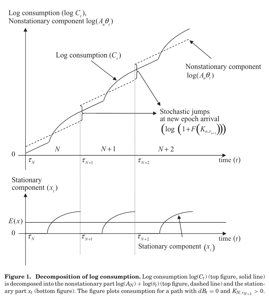
Figure 1 is the picture of this, drawn for the special path with no diffusion shocks ($dB_t=0$), which is why the curves are smooth. The trend line jumps at each arrival; consumption keeps going, then bends up as firms plant; the stationary component traces a sawtooth that sits at zero during the wait and rises concavely afterwards. This is the paper’s main difference from Gomes, Kogan and Zhang (2003), whose cycles come from a trend-stationary productivity process: here consumption keeps a strong random-walk component, and the cycle is the adoption state.

From options to expected returns

Now the asset-pricing step, and it is worth being careful about where it is proved. In the simplified model of Section I there is one epoch and an exogenous stochastic discount factor with a constant interest rate and price of risk. There, for a fixed $\theta_t$, aggregate assets in place are worth $(1+F(K_t))$ times a unit claim and rise with $K_t$, while the growth options are the unexercised calls on $[K_t,1]$ and fall with $K_t$. So the growth-option share of market value falls as adoption proceeds. Lemma 1 adds that the expected excess return on the claim to all growth options is constant and higher than the (also constant) expected excess return on assets in place, for the reason you’d guess: a call is a levered position in its underlying, and in the Internet Appendix’s proof its elasticity to $\theta$ is above one, against one for assets in place. Put the two together and the market’s expected excess return falls with $K$: high early in the cycle, low late. And since early in the cycle is exactly when consumption is furthest below trend and expected growth is highest (eq. 10 makes this exact in the simplified model), you get the signature: when expected returns are high, expected future consumption growth is high too.

Note what is doing the work. Relative risk aversion is constant, $\gamma=9$. Nobody’s appetite for risk moves. What moves is the composition of the market portfolio, which is mostly calls early in the cycle and mostly underlying late in it. It is predictability from leverage rather than from mood.

The full model replaces the exogenous discount factor with a representative agent who has an external habit over the running maximum of aggregate consumption, $M^C_t$, in the Abel (1999) catching-up-with-the-Joneses form, adds recurrent epochs, and makes the planting cost a labour cost. The habit is there to raise the effective elasticity of intertemporal substitution in a growing economy, so the risk-free rate stays low without killing the premium; relative risk aversion stays constant, unlike Campbell and Cochrane (1999). The equilibrium runs on two ratios, the habit ratio $\theta_t/M_t$ and cycle progress $M_t/M_{\tau_N}$. What the paper does not do is prove or simulate the countercyclicality of expected returns in this full model. Footnote 18 asserts that the mechanism “is robust to the determination of the pricing kernel in general equilibrium and the arrival of future epochs”, and points to a discussion at the end of Section III.C that is not in the published text. So Lemma 1 is a simplified-model result, and the general-equilibrium version is an assertion, supported only indirectly by the covariance evidence below.

The paper’s narrative of an epoch (p. 1279) has one twist worth keeping, qualitative as it is. At arrival, before anyone invests, expected growth jumps, so interest rates rise and expected excess returns rise with the new options. Higher rates lower the value of assets in place, so firms with poor draws lose value on the arrival of a new technology, while firms with good draws gain because their options more than offset the rate effect. For the poorly placed incumbents, the good news is bad news. Then the boom comes, and expected returns and rates fall. Why are the options worth anything in general equilibrium at all, given Leahy’s (1993) result that competitive price feedback drives them to zero? Because trees are heterogeneous and not scalable: one per firm per epoch.

The evidence

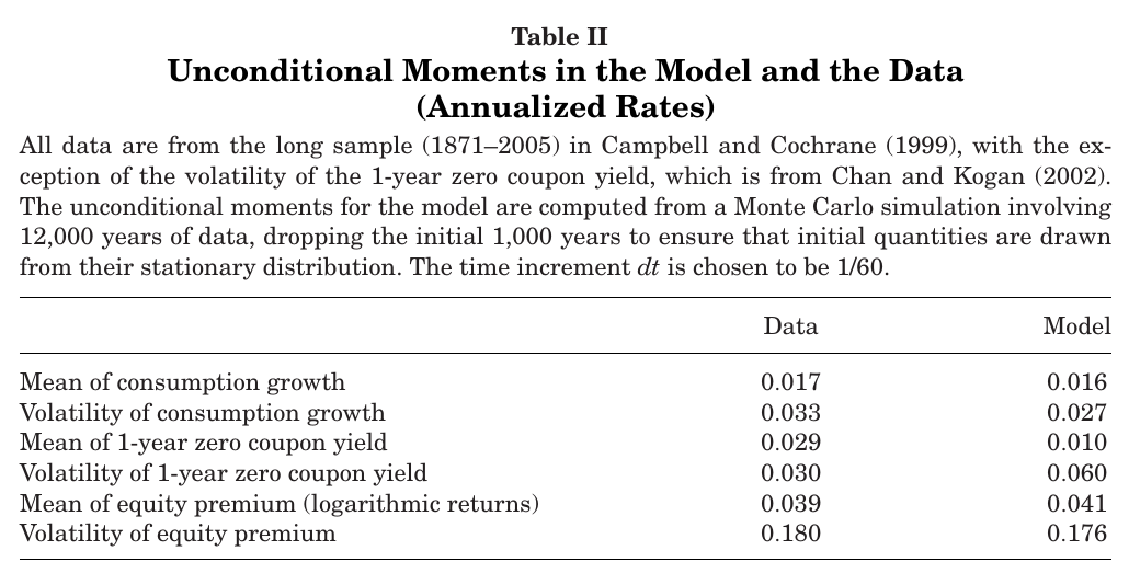
The calibration sets $\lambda=0.1$, a breakthrough a decade, to match Comin and Gertler’s (2006) medium-term cycles; the authors say they are targeting medium-run rather than business-cycle fluctuations. Table II is the usual first exam, and the model passes it at about the level of the endowment habit models it compares itself to. Mean consumption growth is 1.6% against 1.7%, and the log equity premium is 4.1% against 3.9% with volatility 17.6% against 18.0%. The misses are in the risk-free rate, 1.0% against 2.9% in mean and 6.0% against 3.0% in volatility, and consumption volatility is a bit low.

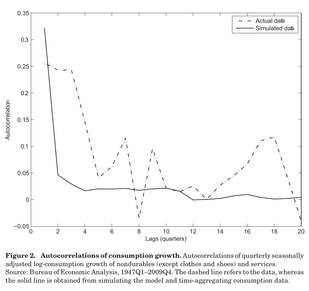
On consumption autocorrelations, the paper says the model’s are “small and decay rapidly”, as in the data, because little of consumption variance comes from the cycle. The picture in Figure 2 is looser than the sentence: the model sits above the data at lag one and then drops off much faster, while the data stay elevated for a few more quarters. Both are small beyond a few lags, which is what “consistent” means here.

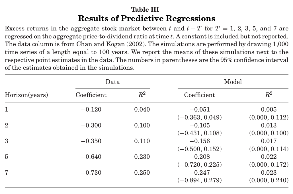
Dividend-yield predictability is there in sign and weak in size. In Table III the model’s coefficients are about a third of the data’s (−0.247 against −0.730 at seven years), and the model’s $R^2$ tops out at 0.023 against 0.25 in the data. All five data coefficients fall inside the model’s simulation bands, but the bands are wide, and the data $R^2$ is outside them at five and seven years. The direction comes from an interesting place: holding the habit ratio fixed, the price–dividend ratio rises with $K$, because depleting options lowers both cash-flow growth and interest rates, and with an elasticity of substitution below one the rate effect wins.

The new test is the one in the abstract. If expected returns forecast consumption growth, then the covariance between this quarter’s excess return and consumption growth cumulated over the following quarters should grow with the horizon, and most of it should come through the expected part of the return:

This is eq. 24 in the paper: $R^e_{t+1}$ is the market excess return over quarter $t+1$ and $\Delta\log c_i$ quarterly log consumption growth, cumulated from $t+3$ to $t+2+T$ (skipping $t+2$ to avoid mechanical time-aggregation overlap), so the first term is the expected-return channel and the second the return-surprise channel.

The point of the split is discrimination between models. In Campbell–Cochrane with i.i.d. consumption the whole covariance is zero. In a habit model with ar(1) predictable growth the Internet Appendix shows the covariances are non-positive, under two conditions on the shock correlations. In Bansal and Yaron (2004) the cumulated covariance does slope upward, but entirely through the second term, because expected returns move only with stochastic volatility. Here it is supposed to come through the first.

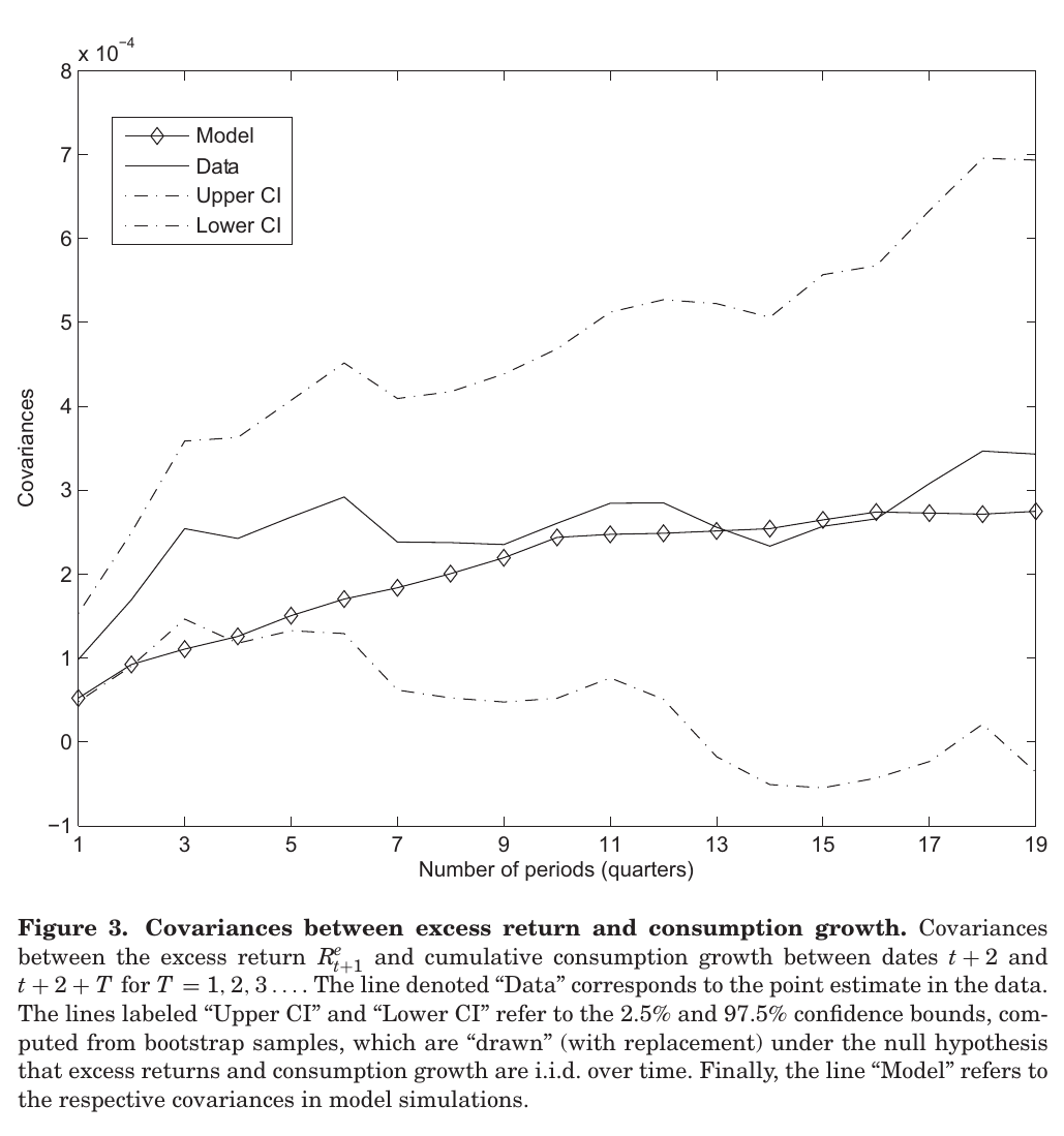
Figure 3 shows that both the data and the model covariances rise with the horizon, from about $1\times10^{-4}$ to about $3.4\times10^{-4}$ in the data over 19 quarters and from about $0.5$ to $2.75\times10^{-4}$ in the model. It is not by itself a rejection of anything: the data line sits inside the bootstrap bands of the i.i.d. null at every horizon. The model line also wanders relative to the data, below the lower band at three quarters, at or slightly above the data around 13 to 16 quarters, and about 80% of the data at 19. It reproduces the slope; the level depends on where you look.

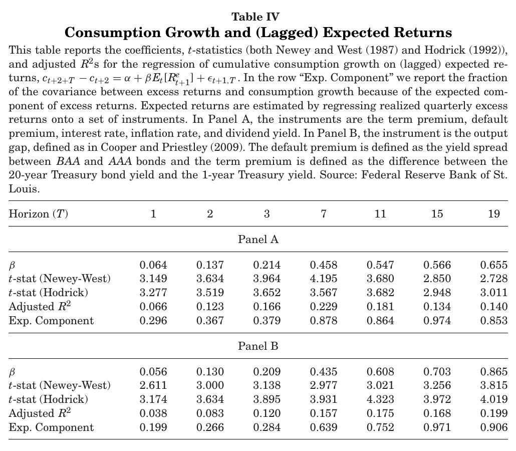
The statistics live in Table IV. Cumulated consumption growth is regressed on fitted expected excess returns, instrumented with the term premium, default premium, short rate, inflation and dividend yield (Panel A) or the Cooper–Priestley (2009) output gap (Panel B). The slopes are positive with Newey–West t-statistics between 2.6 and 4.2 at every horizon. The “Exp. Component” row is the share of the total covariance that runs through expected returns: 0.853 in Panel A and 0.906 in Panel B at 19 quarters, which the text reports as “85%–90% at the 5-year horizon” (19 quarters is the closest column to five years). This is the paper’s main empirical claim, and in data it is a strong one. Inside the model, by contrast, the same share is “slightly above 50%” at five years (0.513 in the Internet Appendix). The model gets the sign and the shape of the decomposition; the data are more expected-return-driven than the model is. Also keep in mind that this is a two-step regression on generated regressors with overlapping horizons, and the answer moves somewhat with the instrument set. The authors are fair about Bansal–Yaron: it could fit if stochastic volatility predicted long-run growth, and they cite Boguth and Kuehn (2010) as finding no such link.

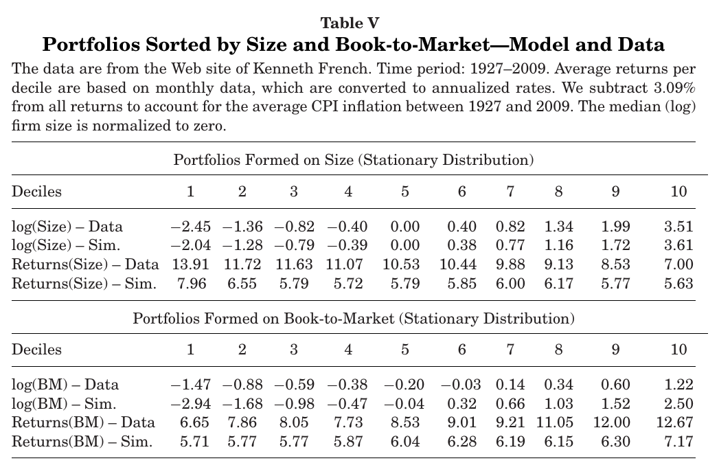
The cross-section follows from the same arithmetic of option shares. Future-epoch options are worth the same to every firm, so among firms that have already planted this epoch, a bigger firm has proportionally fewer options and a lower expected return: a size premium. The value premium looks backwards at first, since high market-to-book should mean lots of risky options, and the resolution is that assets in place are heterogeneous: a firm that has been lucky in its past trees has a higher market value for the same book, so a lower book-to-market and a larger share of its value in safe assets in place. To match the dispersion of size and book-to-market, the authors add idiosyncratic tree shocks, built so that they touch neither the stopping problem, the discount factor nor any aggregate. Table V gets the patterns and about a third to a quarter of the magnitudes: the extreme-decile size spread is about 6.9 percentage points in the data and 2.3 in the model, the value spread about 6.0 against 1.5. “The magnitudes, however, are smaller”, as the paper puts it. And because there is only one priced source of risk, size and value drive each other out in simulations, which the authors flag themselves.

The one surprising thing

The surprising thing is the source of the predictability. Most models that make expected returns move do it by making investors’ risk aversion move: habits in Campbell–Cochrane, volatility in Bansal–Yaron. This one holds risk aversion fixed and lets the market portfolio change composition. A breakthrough fills the market with levered claims on capital that does not yet exist; expected returns go up because the portfolio is more levered, not because anyone is more scared. Consumption has not moved yet, but it will as the options are exercised. That is why expected returns predict future consumption growth here, a link the paper says the leading consumption-based models “face challenges in explaining”, and why the data, where 85–90% of the five-year return–consumption covariance runs through expected returns, are the paper’s best evidence. The side effect is that the arrival of a great technology lowers the value of most existing firms on the day it arrives.

Weak points, my own reading (no discussant exists)

The central theoretical link, expected returns falling as options are exercised, is proved only in the one-epoch model with an exogenous discount factor, and holds there for fixed $\theta_t$; in general equilibrium it is a footnote assertion, and the paper reports no path of expected returns or the option share over an epoch. The model’s expected-return share of the covariance is about half the data’s, P/D predictability is a third of the data’s with tiny $R^2$, the risk-free rate is too low and twice too volatile, and the cross-sectional spreads are a quarter to a third of the data’s. Investment is stylised: the only reason to invest is to adopt the new vintage, investment over output averages 12.4% against 19.9% in the data, and its lowest decile is zero in the model. A back-of-envelope reading (mine, not the paper’s, and dependent on how Table II’s mean growth is measured) suggests the vintage channel adds well under a percentage point of growth a year, against roughly 35 log points if a whole epoch were adopted, so “slow adoption” here may mean most firms never plant a given vintage before the next one arrives. The tractability props are visible too: one tree per firm per epoch, a running-maximum habit chosen for closed forms, and a labour-disutility term engineered so that the planting cost scales properly. The paper’s own register is “can help explain” and “consistent with”, which is right: the evidence makes the endowment benchmarks look worse rather than showing this channel is the true one.

None of which takes away from the idea, which has aged well. Invention is a coin flip, adoption is an option exercise, and the stock market prices the gap between them. If you want to know whether a technology is going to raise growth, the model’s answer is to look at whether the market has got more levered, which is a strange thing to wish for on the day of a breakthrough, and probably correct.

References