The innovation long-run risk component

Fabio Franceschini, Journal of Monetary Economics 163 (2026), article 103987. Published version, with online appendix; no recorded talk.

Fabio Franceschini’s paper takes on the long-run risk model’s oldest problem, which is that its persistent component of expected consumption growth is very hard to find in the data. Bansal and Yaron (2004) need a small, slow-moving drift in expected growth that investors fear a great deal, and the obvious objection is that you can make an Epstein–Zin (1989) investor fear anything you can’t measure. Kung and Schmid (2015) gave the drift a physical source: R&D. Firms invest in ideas, ideas raise productivity for years, so a burst of R&D today is news about the whole future path of consumption. That is a nice story. It is also a story about a variable that, measured the obvious ways, turns out to have a unit root, which is an awkward property for something meant to be the stationary engine of expected growth. The paper’s job is to find the version of R&D that actually behaves like that engine, pull shocks out of it, and see whether markets price them.

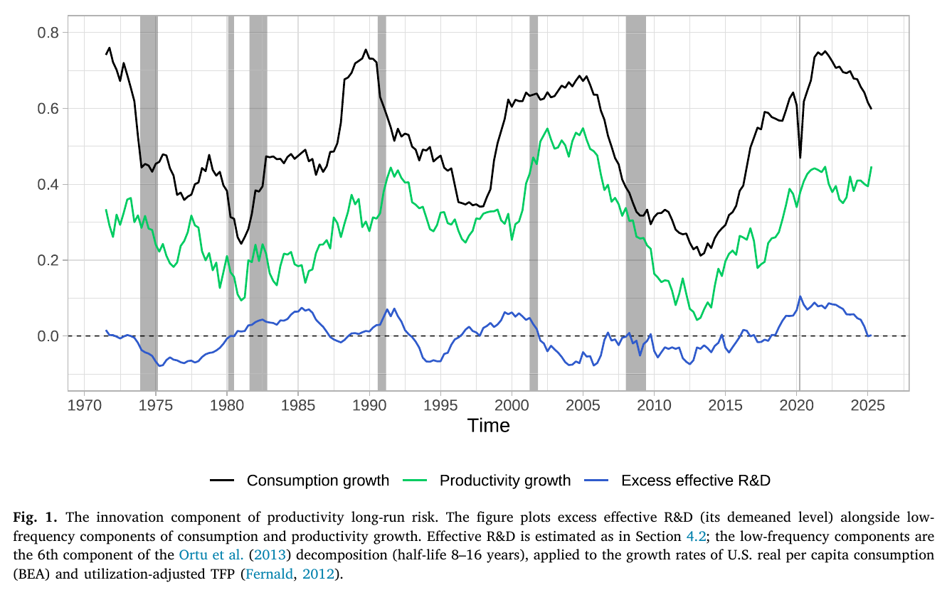
Fig. 1 is the pitch: the paper’s cleaned R&D series alongside the slow (8–16-year half-life) components of us consumption and tfp growth, with lows in the late 1970s, the mid-1990s and 2003–13. It looks good, and there is no statistic attached to it. It shows what the author hopes is true. The test comes later.

The mechanism: R&D measured in units of growth

Start with a Jones (1999)-style lab-equipment economy. Output is $Y = ZL$, tfp is $Z = I^{\theta} Q^{\xi} e^{a}$, where $I$ is ideas per variety, $Q$ is the number of varieties, and $a$ is a stationary non-technological process (misallocation, public R&D, utilisation leftovers). New ideas come from spending $S$, but with two drags: spending is spread across more and more varieties, and, when spillovers are less than one for one, each new idea is harder to find given the stock you already have. Log-linearise the growth of $Z$, and expected tfp growth turns out to be linear in exactly one transform of R&D spending:

This is eq. 10 in the paper: $S_t$ is aggregate R&D, $I_t$ average ideas per variety, $Q_t$ product variety, $\psi$ the spillover from past ideas net of fishing-out, and $\eta$ the duplication elasticity, so $s_t$ is R&D expressed in units of expected productivity growth.

The paper calls this “effective R&D”, and the point is the second and third terms. To hold growth constant you have to keep raising spending in line with the idea stock and variety, and the author puts the punchline nicely: any lower level of investment, “however high in absolute terms”, means falling effective R&D and slowing growth. It is the only transform of $S$ with this linearity in both the fully endogenous and the semi-endogenous regimes, which is why R&D growth and R&D over gdp are rejected as measures (R&D/gdp coincides with effective R&D only under the special fully endogenous restriction, which the data go on to reject).

Now the clever bit. tfp growth is stationary, so $s_t$ must be stationary. But $\ln S$, $\ln I$ and $\ln Q$ all trend. So $s_t$ is a cointegrating residual, an error-correction term, and the economics says why: R&D cannot permanently outrun the frontier, because R&D builds the stock that makes the next dollar of R&D less effective. Deviations of $s_t$ from its mean drive expected growth, and if those deviations follow an ar(1) with persistence $\rho_s$, an innovation $\tilde\varepsilon_t$ is news about the entire future of productivity:

This is eq. 14 in the paper: $Z$ is tfp, $\gamma_1$ the loading of tfp growth on effective R&D, $\rho_s$ the persistence of excess effective R&D and $\tilde\varepsilon_t$ its shock, so persistence multiplies the long-run news and with it the variance of the consumption news an Epstein–Zin investor prices.

That is the long-run-risk transmission in one line. The more persistent the error-correction term, the bigger the price of risk. (The author flags the obvious tension himself: the mechanism is strongest exactly where stationarity is hardest to establish.)

You can’t see $I$ or $Q$. So the paper swaps them for things you can: $I$ for tfp via the production function, and $Q$ for employment via $\ln Q_t = \omega \ln L_t + \pi a_t$. The residual of a cointegrating regression of $\ln S$ on $\ln Z$ and $\ln L$ is then “gross effective R&D”, and “gross” here means contaminated, not pre-depreciation: because $\ln Z$ contains $a_t$, the residual inherits a negative loading on the non-technological process. (The printed coefficient on that contamination and the one implied by the online appendix’s own derivation disagree on a sign inside it. They coincide when $\pi = 0$, and the contamination stays negative either way.) The cleanup is a bivariate var in tfp growth and the residual, identified with one timing assumption, that R&D moves real quantities only with a lag:

This is eq. 26 in the paper: $\boldsymbol w_{x,t}$ are the var residuals ordered tfp growth first and the effective-R&D measure $x_t$ second, and the zero says the R&D shock $v^s_t$ cannot move tfp on impact, so $v^a_t$ and $v^s_t$ recover the non-R&D and R&D shocks whichever measure $x$ is used.

The Cholesky triangle does two jobs at once: it strips the $a_t$ leak out of the residual, and it purges R&D surprises of contemporaneous tfp. What is left, $\varepsilon^s$, is whatever moves R&D but not tfp today. The author is candid that this is not “fundamental in an absolute sense”, and that financial conditions could be in it.

The evidence

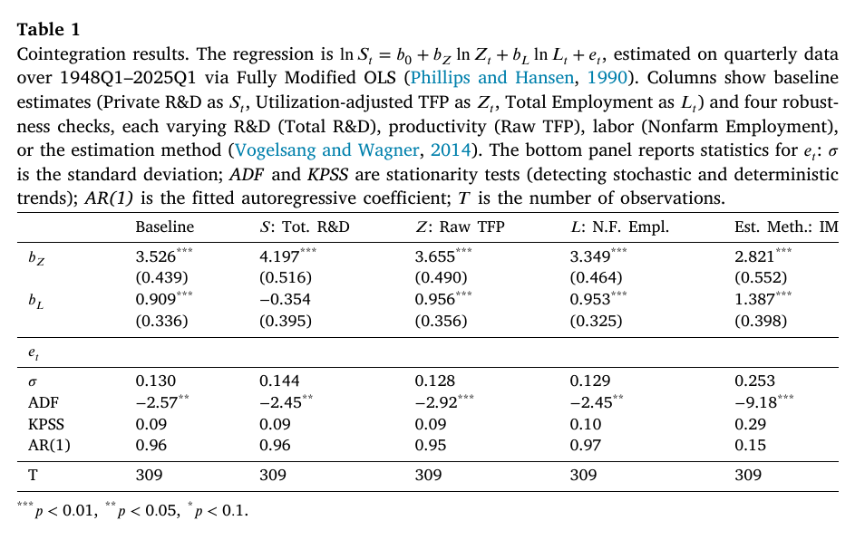
Quarterly us data, 1948Q1 to 2025Q1: real private R&D, Fernald’s (2012) utilisation-adjusted tfp excluding R&D capital, and total employment. In Table 1, fm-ols gives $b_Z = 3.526$ (s.e. 0.439) and $b_L = 0.909$. The residual has adf −2.57, passes kpss, and has ar(1) 0.96, which is persistent enough to matter and stationary enough to use. The 3.5 is quietly important: a fully endogenous balanced growth path needs $b_Z = 1$, and this rejects it at any level. So the paper backs innovation long-run risk while rejecting the fully endogenous version of the model family that motivated it. Long-run risk here means long transitional swings in growth and a permanent shift in levels, not a permanently higher growth rate. In the online appendix, the Kung–Schmid ratio of R&D to the R&D stock behaves like a near-unit-root process with a half-life measured in decades, and the author’s “likely” explanation is that fixing spillover strength rather than estimating it is what fails.

From the text: one standard deviation of gross effective R&D predicts about 0.8% a year of extra tfp growth, close to Kung and Schmid’s calibration, with implied half-lives between 2 and 20 years at 95%. A second step recovers a “net” series that strips $a_t$ out directly. It is cleaner, but it costs five more assumptions ($\eta = \omega = 1$, $\pi = 0$, $a_t$ spanned by macro factors, no one-period-ahead feedback from R&D into labour or $a_t$).

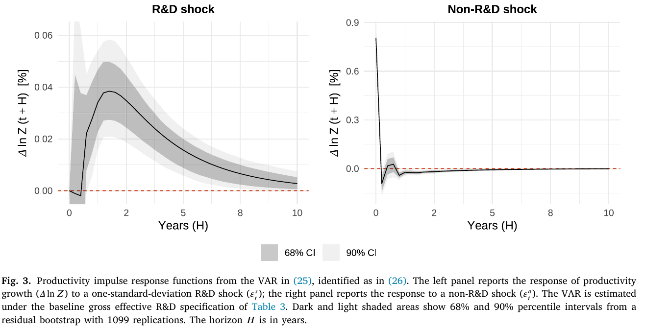
Fig. 3 is the macro result, and it has the right shape. The non-R&D shock does almost all its work on impact and is gone within five years. The R&D shock does nothing significant for a year, humps (the text says it peaks at two years; on the plot it is closer to a year and a half), and its 90% band still excludes zero at ten years. The peak is small, around 0.04 percentage points of quarterly tfp growth, but it lasts, and lasting is what the theory asks for.

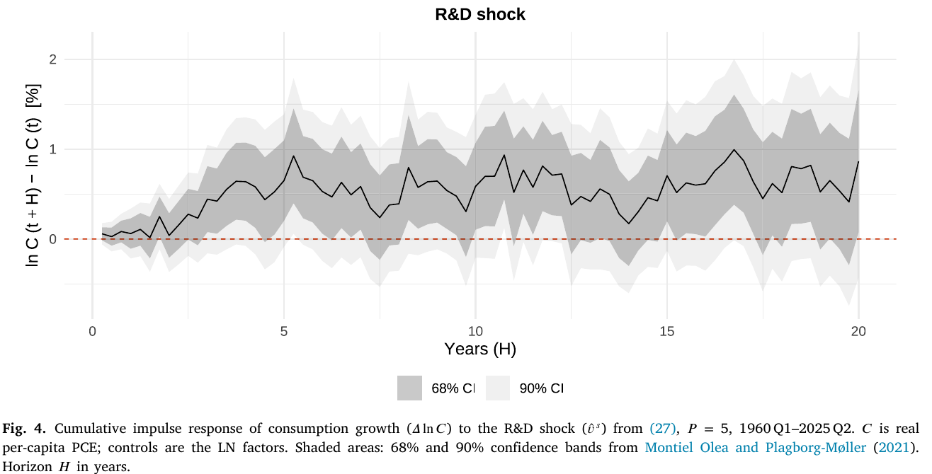
Consumption, in local projections out to 20 years, rises slowly for about six years and then plateaus at roughly half a percent to one percent of the level. That is consistent with a persistent or permanent level shift. It reaches 68% significance only after about three years, and the 90% band touches zero at many horizons. The plateau is also what lets the local-projection coefficient stand in for long-run consumption news: if the response is flat from some horizon on, the cumulative response is the discounted sum.

The one surprising thing

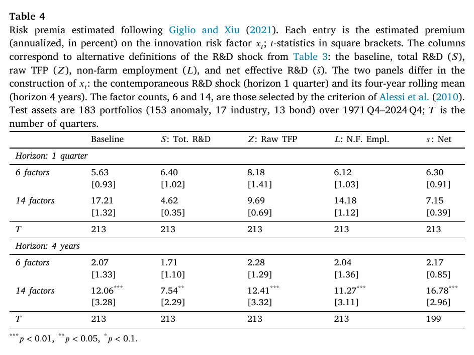
Now the pricing. The logic is tidy: $\varepsilon^s$ carries long-run consumption news and a negligible contemporaneous consumption surprise, so its premium prices long-run risk alone. It is estimated with Giglio and Xiu’s (2021) three-pass method on 183 test assets (153 anomaly portfolios, 17 industries, 13 bond portfolios), 1971Q4 to 2024Q4, so that omitted factors don’t bias it.

Here is what Table 4 actually says. The R&D shock itself, the object the whole model says investors should price on arrival, has a positive premium that is not distinguishable from zero. The t-statistics are all below 1.5, and with 14 factors the point estimate is 17.21% at t = 1.32. The number in the abstract, “around 12% annually”, belongs to a different factor: the four-year rolling mean of the shocks, which earns 12.06% a year (t = 3.28) with 14 latent factors. With 6 factors the same rolling mean earns 2.07% at t = 1.33. The paper’s bridge between the two is investor under-reaction to R&D news, imported from Eberhart, Maxwell, and Siddique (2004), who find under-reaction lasting up to five years.

So the headline evidence for a rational Epstein–Zin model of news pricing depends on investors being slow to price the news. That may well be true, and a small slow-diffusion story bolted onto a long-run-risk model is hardly the strangest thing in asset pricing. But it means the 12% is a statement about a smoothed factor plus an under-reaction story, not about the shock the model defines. And one cell being insignificant while another is significant does not show the two differ.

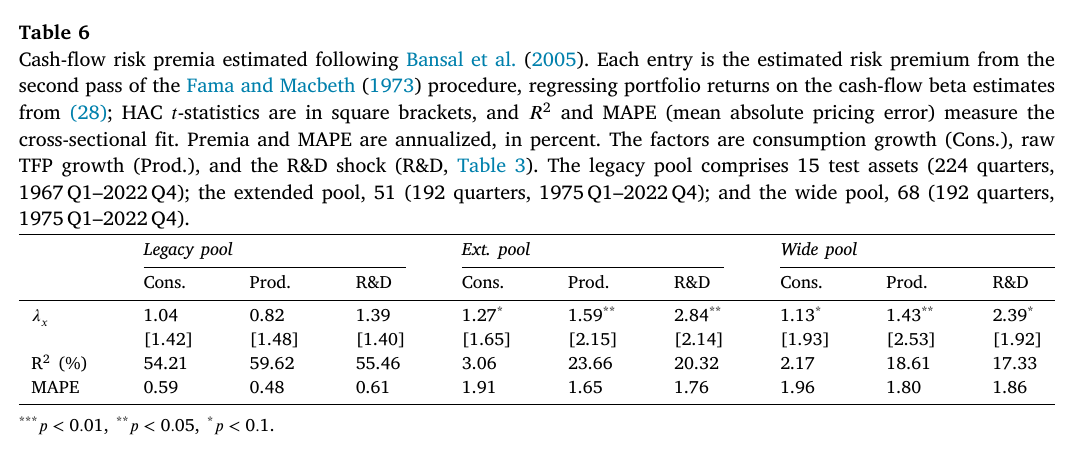
The cash-flow test is the paper’s answer to “is this really fundamentals?” Following Bansal, Dittmar, and Lundblad (2005), portfolio dividends are regressed on an eight-quarter moving average of the shock, and the betas are priced with the consumption price set to zero. Small, R&D-intensive and profitable firms load positively, and big firms barely move. In Table 6 the R&D cash-flow premium is 2.84% (t = 2.14) in the extended 51-asset pool and the highest of the three in every pool. It is not significant in the original 15-asset pool, though, and productivity fits the cross-section better everywhere. The author’s own phrasing is fair: the R&D cash-flow premia are “only a fraction of the return-based premia”. Different estimator, factor, assets and sample, so don’t turn that fraction into a share explained.

Weak points, my own reading (no discussant exists)

The rolling-mean factor is a researcher choice. A 16-quarter overlapping average over 213 quarters leaves few independent observations, and a smoothed series could proxy for any slow-moving priced state, so I would want to see it across window lengths. Identification is Cholesky with tfp first, so news about future tfp from anywhere else would also move R&D now and tfp later. A delayed hump, which is what Fig. 3 shows, is also what a news shock looks like. The var explains little of tfp growth, the R&D residuals are strongly heteroskedastic, and the bands come from a residual rather than wild bootstrap. The cointegration adf of −2.57 is starred without saying which critical values are used, and Engle–Granger (1987) values for three variables sit well below that. The gross and net shocks are supposed to be identical in theory but correlate well short of one in the online appendix. The paper’s Table 5 big-firm rows also appear swapped relative to the online appendix’s version. Finally, there is no calibrated Epstein–Zin model asked to match both the macro responses and the premium. The paper shows persistence and a positive price and calls that consistency, which is fair as far as it goes. It stops short of a premium that has to come out right.

All of which leaves the paper in an honest and useful place. It has built the right measuring stick for R&D as a growth engine, found that it moves productivity for a decade, and found that markets care about it eventually, roughly the way they care about most good news from the lab.

References