Are We Fragmented Yet? Measuring Geopolitical Fragmentation and Its Causal Effects

Jesús Fernández-Villaverde (University of Pennsylvania, CEPR, NBER), Tomohide Mineyama (International Monetary Fund) and Dongho Song (Johns Hopkins University), “Are We Fragmented Yet? Measuring Geopolitical Fragmentation and Its Causal Effects,” dated February 4, 2025, 65 pages including the online appendix; circulated as NBER Working Paper 32638 (June 2024, revised February 2025) and CESifo Working Paper 11192, and not published in a journal at the time of writing. This is written from the February 2025 revision. No recording of a presentation of this paper exists, so there is no talk, no discussant and no Q&A to draw on; everything below comes from the manuscript, and Figures 2, 3, 7 and 8 and Table 1 are cropped from it.

You would like to know whether the world economy is coming apart, and you would like to know it as a number. This is harder than it sounds, in an annoying and specific way. Trade as a share of world GDP has been roughly flat since 2008, which sounds like nothing much happening. The count of trade-restricting measures nearly tripled between 2019 and 2022, which sounds like a great deal happening. Sanctions in force have risen more or less monotonically for four decades; the Global Sanctions Data Base counts 1,325 of them enforced since 1949. Cross-border patent flows have thinned. Countries vote less alike at the UN General Assembly. Every one of these numbers measures something real, none of them measures “fragmentation,” and the moment you pick one you have quietly picked your answer.

The usual escape hatch is to average several of them, which is worse, because now you have chosen weights and pretended you didn’t. The authors say this plainly: choosing one indicator, or an average of them, “can be arbitrary and may lead to incorrect conclusions or policy recommendations.” So they do the thing econometricians do when the object of interest is not observable and the observables are all partly about it. They declare fragmentation a latent variable, gather sixteen indicators as noisy proxies, and let a likelihood function decide how much each proxy is worth.

What the model actually is

Sixteen quarterly series, 1975 through the first quarter of 2024, sorted into four groups. Trade gets five, including trade openness, the count of trade restrictions and trade policy uncertainty. Financial gets three: foreign direct investment, portfolio and other investment, and a capital-control index. Mobility gets three: net migration, cross-border patent flows and a newspaper-based migration fear index. Politics gets five: geopolitical risk, energy uncertainty, a count of international conflicts, the count of sanctions in force and the UN voting-alignment score. Everything is standardized, and the five series where more means integration are multiplied by minus one, so that up is always bad.

Then a dynamic hierarchical factor model, which is a phrase that deserves to be forced to say what it means. It means exactly two levels. Each of the sixteen indicators loads on its group’s factor; each of the four group factors is the sum of one world factor and that group’s own private wedge. In the paper’s equation (2):

Indicator $k$ inside group $j$ — trade, financial, mobility or political — at time $t$ is a deterministic trend $a^{(j)}_{k,t}$, plus a time-varying loading $b^{(j)}_{k,t}$ on the world fragmentation factor $f_t$ scaled by $\lambda^{(j)}$, plus that same loading on the group’s own wedge $\eta^{(j)}_t$, plus a serially correlated idiosyncratic error. The group factor itself, equation (3), is a random walk hit by two shocks whose volatilities are themselves random walks:

The common innovation $\epsilon_{f,t}$ passes into every group with weight $\lambda^{(j)}$; the group’s own innovation $\epsilon^{(j)}_{f,t}$ is what makes it different from the world. The stochastic volatility is there so that 1991, 2008 and 2020 can be loud quarters without permanently rescaling the model’s sense of what a normal quarter looks like. Kill the group innovations and you have an ordinary one-factor model; kill the common one and you have four unrelated indices.

The wedge is the whole point of the exercise. It lets the paper say, in a single estimation, both “here is one number for fragmentation” and “here is what politics is doing over and above that number.” That second sentence is where the interesting result lives, and you could not get it by running four models and squinting.

It is worth being honest about what is estimated and what is imposed. Identification comes from hard normalizations: the initial loadings are set to 0.5, the common innovation variance to 1, each group innovation variance to 0.1 — group shocks are assumed one-tenth the size of common ones — and $\lambda^{(j)}=1$ for all four groups, which assumes that the world factor passes one-for-one into every group. The paper’s stated “key finding” is that “substantial comovement exists across groups.” Some of that comovement is a normalization wearing a finding’s clothes. What is genuinely estimated is the wedge, and happily the wedge is the good part.

Three phases, and a credible interval nobody wants to look at

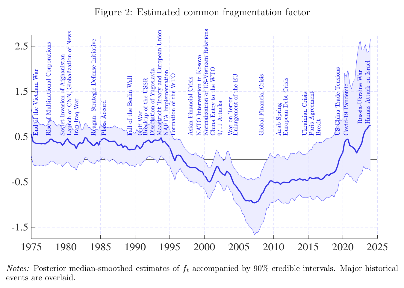
Out comes a story you already half-believe, which is both reassuring and slightly suspicious. Flat from 1975 to the early 1990s, when the world was divided into blocs and stayed that way. Falling — globalizing — from about 1995, with the Soviet collapse, Maastricht, the WTO, China’s accession. Rising after 2008, accelerating from 2017 to 2020, pausing in 2021–22, and surging from 2022 with Ukraine and the Hamas attack. The paper’s summary is that fragmentation “has increased to its highest levels in the sample, with no signs of reversal.”

That sentence is a statement about the posterior median. The median ends the sample near +0.7. The 1975–93 plateau sits near +0.4 to +0.5. And the 90% credible interval at the end of the sample runs from roughly −0.2 to +2.6. So the claim that today is the most fragmented moment in fifty years is not, at 90% credibility, distinguishable from the mid-1970s — or from zero. This is not sloppiness so much as physics: $f_t$ is a driftless random walk with stochastic volatility, so posterior uncertainty is mechanically widest at the endpoint, which is precisely where the paper’s motivation lives. Anyone quoting “highest ever” should carry the band along with it.

The thing everybody is measuring is not the thing that is happening

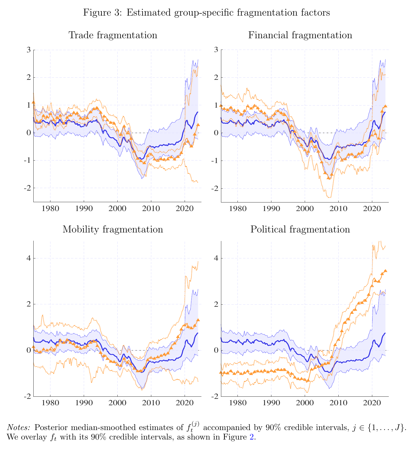
Here is the finding that should reorganize how you read the deglobalization literature. The public conversation about fragmentation is a conversation about trade — tariffs, the 2018-19 trade war, friendshoring, supply chains. Every number in the newspapers is a trade number. In the decomposition, trade is the tamest of the four groups. It fell below zero only around 2005, a full decade after the common factor turned in 1995. It did not accelerate after 2008. It has risen “over the past eight years,” and it ends 2024 roughly back where it started, still below its own early-1990s level. The authors’ own reading is that looking only at trade would tell you this is “slowbalization” rather than fragmentation, and the group factor agrees: on the trade dimension, the world has un-globalized, not fragmented past its Cold War state.

The political factor sat around minus one for the first twenty-five years of the sample — below the common factor, which is to say the world was politically more integrated than it was integrated generally. It crosses the common factor around 2008 and runs to roughly +3.5 by 2024, against a common factor of about +0.7. Sanctions, conflicts and geopolitical risk are doing essentially all of the work of dragging the headline index to its record. Financial fragmentation tracks the common factor almost one-for-one, with more volatility, which makes it less a separate dimension than a restatement of the index. Mobility shows no significant idiosyncratic movement at all and has bands wide enough to drive a container ship through.

Turning an index into a percentage of GDP

The second half of the paper takes the estimated factor and asks what a shock to it does. There is a panel SVAR with eleven variables — the fragmentation index plus the VIX, the S&P, oil, the two-year Treasury, financial conditions and world GDP, which is deliberately the Caldara–Iacoviello variable list, plus four country variables — and separately a panel local projection, equation (6):

The cumulative $h$-quarter change in country $i$’s log GDP per capita, industrial production, fixed investment or stock price, regressed on the fragmentation shock $s_t$ recovered from the SVAR, with two lags of the outcome and of the shock, a global and country control vector $X_{i,t}$, and country fixed effects $\mu^{h}_{i}$. The sequence of $\beta^h$ is the impulse response. The LP samples are large — 6,962 country-quarters for GDP per capita across 36 advanced and 53 emerging economies — and the VAR’s are not, at 2,359 observations from 26 countries, because a VAR needs everything at once.

Everything then rides on identification, and the honest description is that the baseline is a recursive ordering with fragmentation first. That assumption says fragmentation is driven by low-frequency forces — demography, ideology, “legislative and engagement processes” — so it cannot respond within the quarter to global GDP, oil, the VIX or financial conditions. As a stress test they also order it last, which assumes it affects nothing contemporaneously, and call that the worst case.

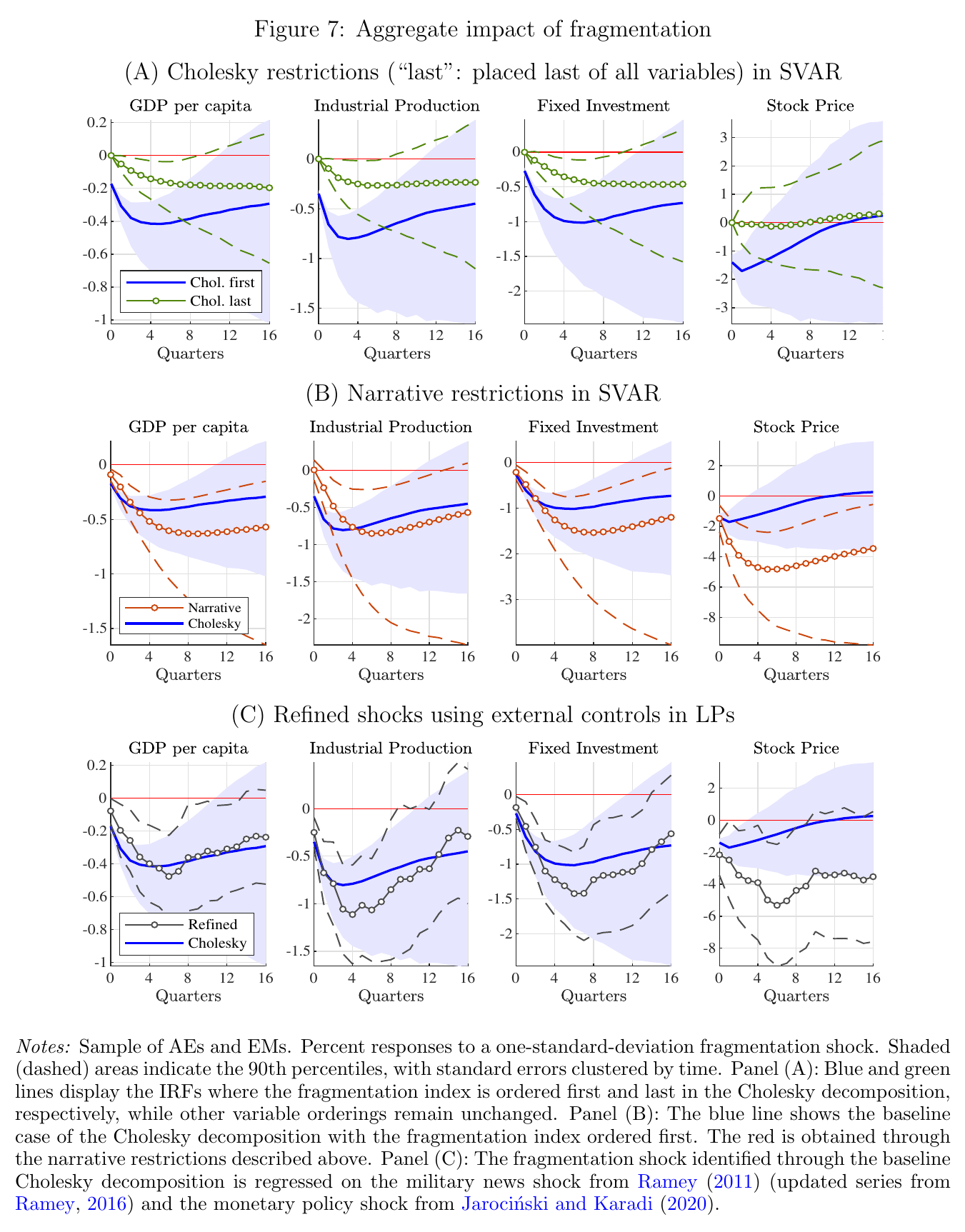
A one-standard-deviation fragmentation shock cuts GDP per capita by about 0.4% at the trough, five or six quarters out, and is still about 0.3% down after four years. Industrial production troughs near −0.8%, fixed investment near −1.1%, stock prices near −1.7% on impact. Under the worst-case ordering the GDP effect halves to about −0.2%, industrial production to −0.3%, investment to −0.5%, and stock prices lose significance entirely, which the authors attribute to equities being forward-looking. Under the narrative instrument the GDP effect roughly doubles to 0.7%, and the authors read the amplification as classical measurement error in the index being corrected by the instrument. Bear in mind that “one standard deviation” is a normalization of a unitless latent variable; it is not a percentage of anything.

Emerging markets, asymmetry, and the sectors

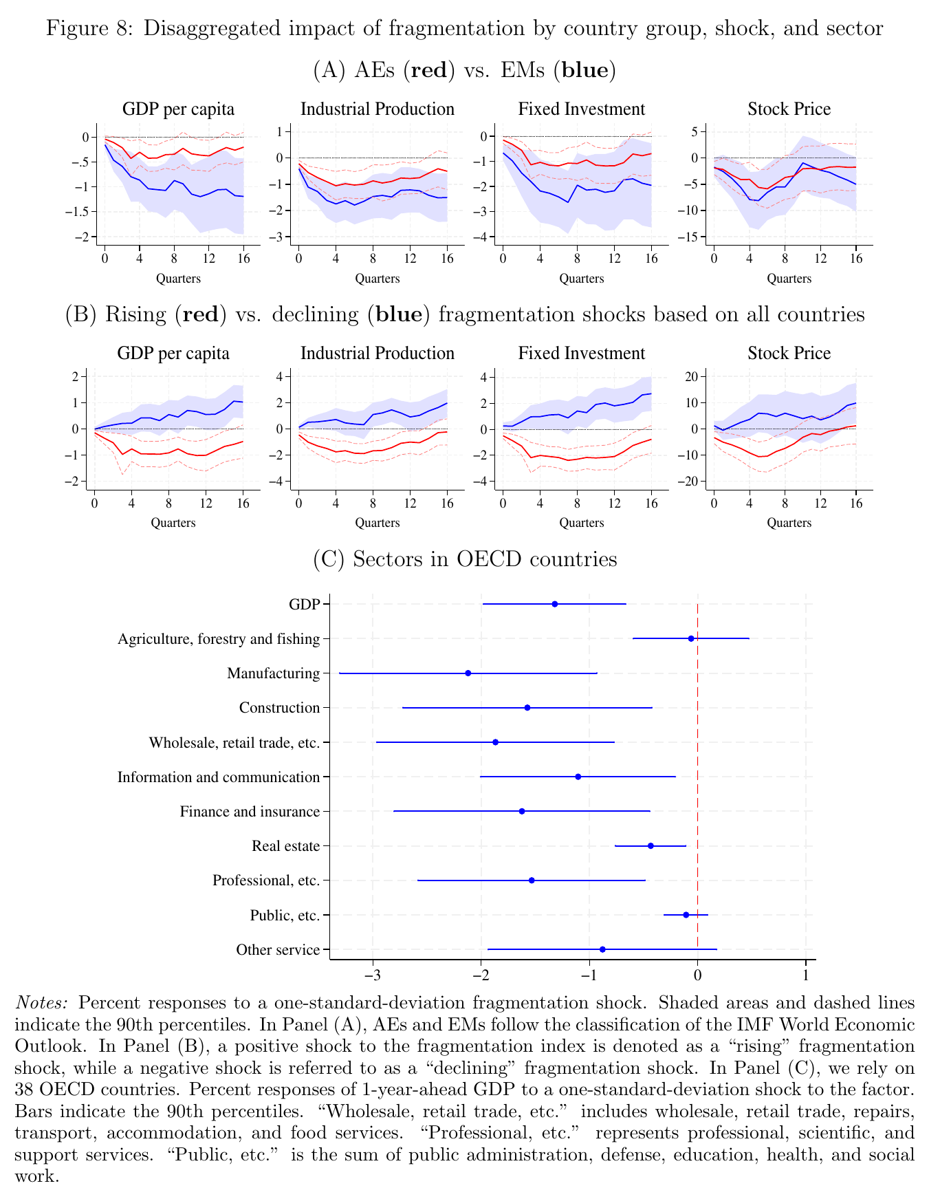
Advanced economies lose between 0.2% and 0.4% of GDP per capita and are back near −0.2% at the four-year horizon. Emerging markets decline steadily to about −1.2% and are still falling when the horizon ends. Fixed investment in emerging markets troughs near −2.5%. This is the least surprising result in the paper and also the one with the clearest policy content: the countries that were going to catch up by integrating are the countries that pay when integration stops.

The asymmetry is the paper’s favorite finding, and it is genuinely striking. Rising and falling fragmentation shocks are estimated in separate projections. Rising fragmentation costs about 0.9% of GDP per capita within four quarters and stays there. Declining fragmentation — globalization — builds slowly and monotonically and reaches about +1.0% only at the sixteen-quarter horizon. Stock prices fall about 10% within five quarters on the way up and gain about 9% over four years on the way down. Put in the least flattering way available: you pay for fragmenting this year and get repaid for opening up over half a decade, which is a payoff profile no politician has ever been observed to choose voluntarily.

The sectors behave about as you would guess, with one wrinkle. In a one-year-ahead projection across 38 OECD countries, manufacturing takes roughly −2.15% against aggregate GDP at about −1.35%, with distribution and transport at −1.85%, construction, professional services and finance clustered near −1.55%, and agriculture and public administration indistinguishable from zero. The paper reads this as global-facing sectors versus insulated ones, but the dichotomy is imposed on a gradient: professional and scientific services, which nobody would call trade-exposed, get hit about as hard as finance, and real estate is significantly negative at about −0.45% while sitting in the “insulated” bucket.

The nulls are the interesting part

Then the paper orthogonalizes the group shocks, so that a trade-specific shock is one that moves the trade factor without moving the common factor or any other group factor. Almost everything goes away. Trade-specific shocks produce an initial dip that fades within a few quarters. Financial-specific shocks come out with a positive sign on impact, which is the wrong sign, and is attributed to the orthogonalization. Mobility does nothing except to stock prices. Political fragmentation shocks are the sole exception: persistent, additional negative effects on the global economy, with equities hit hardest, which the authors tie to wars, conflicts and sanctions.

So both halves of the paper point the same way. The measured fragmentation is political, and the measured damage is political. The instruments governments actually control and argue about — tariffs, trade restrictions, industrial policy — are not where the index moved and not where the damage came from. Trade policy cannot fix the part that hurts, and trade economists do not model it.

The bloc result is stranger still. Splitting the indicators into a U.S.-EU bloc, a China-Russia bloc and everyone else, shocks to U.S.-EU fragmentation damage the global economy immediately and shocks to the “Others” bloc damage it in the medium run, while China-Russia fragmentation shocks show no significant effect at any horizon examined. The bloc whose decoupling is the entire subject of the geoeconomics literature is the one that does not register. The authors offer two readings and tell you to be careful with both: that China’s expansion increased competition and substituted for other suppliers, and that their framework may not capture spillovers, since the 2018-19 trade war relocated trade from China to Mexico and Vietnam and thereby diluted the measured impact. That second hedge is itself a result — it is Gopinath’s “neutral bystander” story appearing in the data as an econometric null.

Where a referee would push

The first and cleanest objection is that a generated regressor is being treated as data. The fragmentation index is a posterior estimate with credible bands wide enough that its terminal value is not distinguishable from zero, and its innovation is then dropped into the SVAR and the local projections as though it had been observed. There is no propagation of the Gibbs posterior draws into the impulse-response bands, no bootstrap over factor draws; the reported 90% bands are conditional on the median factor. Given the width of those bands in the index chart above, this is not a nitpick, and it is the single easiest thing to demand.

The second is that the baseline identifying assumption sits badly with the basket it identifies. Ordering fragmentation first requires that the index cannot respond within the quarter to global GDP, oil, the VIX or financial conditions, on the grounds that legislatures and diplomats are slow. But five of the sixteen indicators are ratios whose denominator is contemporaneous GDP, and four are text-mining indices built from newspapers, which move within days of a market event. A global downturn collapses trade faster than it collapses GDP, mechanically lowering measured trade openness and therefore mechanically raising measured fragmentation in the same quarter. That is precisely the reverse causality the ordering assumes away. And the paper tells you what it costs: under the ordering that shuts the channel off, the GDP effect halves and stock prices lose significance. Half the headline number rides on an assumption that the construction of the index partly contradicts.

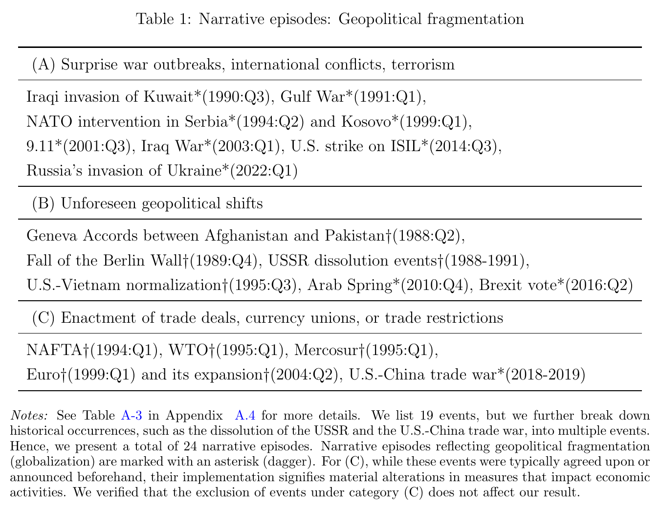
The third is the narrative instrument, which is offered as the answer to exactly that worry and is not strong enough to be one. The correlation between the reduced-form residuals and the narrative series is about 0.15. The first stage is a coefficient of 0.080 with a clustered standard error of 0.030 — a t-statistic around 2.7, an implied first-stage R-squared of roughly 2%, no F statistic reported, no weak-instrument-robust bands. And look at what the episodes are: the Iraqi invasion of Kuwait, the Gulf War, Serbia, Kosovo, 9/11, the Iraq War, ISIL, Ukraine. Those are oil shocks and military shocks, with large direct macroeconomic effects that need not travel through anything called geopolitical fragmentation at all. The narrative estimate comes in at nearly double the recursive one, and the authors read the gap as measurement error being corrected. The equally available reading is that the instrument has picked up the oil price and defense spending. Tellingly, the paper’s “refinement” exercise — partialling out Ramey’s military news shock and the Jarociński–Karadi monetary shock — is applied to the recursive shock, not to the narrative one, which is where that particular cleaning would have bitten. A further twenty-four episodes hand-coded plus-one or minus-one across 136 quarters is a small enough instrument that a handful of recodings is the whole thing, and some of the codings are arguable on their face: the Arab Spring is coded as fragmentation, though it was widely read at the time as democratization.

The fourth is a matter of sample. The local projections stop at 2019:Q4, so that the sample is consistent across horizons. That is a defensible choice with an awkward consequence: every event in the paper’s own opening paragraph — Ukraine, the Hamas attack, the 2022 surge in trade restrictions — is outside the window in which the cost of fragmentation is estimated. The causal half of the paper is identified off 1990s wars, 1990s trade deals and the 2018-19 trade war, and then applied rhetorically to a post-2022 world. The same window problem shows up inside the index: tariffs end in 2014, UN voting alignment in 2015, capital controls and patents and temporary trade barriers in 2019. The surge that motivates the whole enterprise is measured by the subset of indicators that still report, several of which are text indices built from American and Western European newspapers. The model handles missing data formally and honestly; it cannot manufacture information that is not there, and the widening of the bands at the right edge of the chart is the model saying so.

There is also a small piece of surgery worth flagging, mostly because of what it says about the genre. The projections include a dummy for 1996:Q1, because the SVAR produced a 3.3-standard-deviation fragmentation shock in that quarter “that lacks a clear economic narrative.” Dropping an observation because you cannot narrate it is a narrative judgment, inserted into a procedure whose stated advantage is that it “minimizes the subjective decisions a researcher needs to make.”

None of which is fatal, and the paper is better than most of what is written on this subject precisely because it puts its normalizations, its worst-case ordering and its own weak first stage on the page where you can find them. The place it lands, though, is not quite the place the title implies. Ask “are we fragmented yet” and the honest answer from this index is that the median says yes, the credible interval declines to commit, the trade dimension that everyone argues about has barely moved past where it was during the Cold War, and the part that is unambiguously fragmenting — sanctions, conflicts, geopolitical risk — is the part that no trade agreement has ever been able to reach. Which may explain why the conversation stays on tariffs. They are the part you can hold a vote about.