Generative AI and Pre-Hire Labor Market: Evidence from a Chinese Job Matching Platform

Hanming Fang, Jiayin Hu, Miao Yu and Jiaqi Zhao; presented by Fang at the nber Economics of Artificial Intelligence conference (Fall 2026, Toronto), day 2, 24 September 2026; discussant Lindsey Raymond (mit). There is no public draft, so this is written from the talk and slides alone.

A job posting in China has a feature that a job posting in the us mostly does not: a line promising that you get your weekends off. Fang put it plainly: “if a company can guarantee weekends off they will make that as a very desirable feature in their job posting. If that’s not mentioned then you can expect that you may be asked to work overtime or on weekends” (01:37:14). Only 19% of postings on the platform make that promise (01:37:43). Average weekly hours are 48, according to the slide (01:29:17). So an employer who wants to make a job worse has two dials: the monthly wage, and whether to mention Saturday.

Now suppose your occupation becomes more automatable. You would expect the employer to post fewer of these jobs, and to post lower wages on the ones it keeps. What this paper says is that the employer also turns the second dial. For more senior postings, the second dial moves more than the first. Most of what is interesting here comes from that second dial, and so do most of the questions about whether the result is true.

The setup

The data come from “one of the largest online recruitment platforms in China,” which the talk does not name (slide at 01:31:54). On the employer side there are 200,000 random postings a year for 2021–2024. After cleaning, that leaves 777,718 postings across 183 industries and 93 second-level occupations. The sample ends before DeepSeek (01:32:17). On the applicant side there are two samples (slide at 01:33:43). One takes 15,000 positions a year with every application each received. The other takes 20,000 job seekers a year with their full application histories. The key outcome is the “callback,” a positive reply from the employer within 24 hours: an interview scheduled, a phone call, an exchange of contact details, or continued chat. The platform does not record whether anyone was actually hired (01:34:34). So the callback is, as Fang said, “the best we can do.”

Treatment is the familiar continuous difference-in-differences. The exposure measure is an occupation-level llm exposure index in the Eloundou et al. tradition. It was adapted to China by Zhang et al. (2025), who re-weight tasks by their importance in 1.25 million postings from the same platform. The measure is interacted with a Post dummy that switches on in December 2022, the month after ChatGPT’s release. The posting-level specification, from Fang’s slide at 01:38:42, is

Here $g(j)$ is the posting’s occupation. The model includes year-month, job-city and detailed-occupation fixed effects, and standard errors are clustered by occupation type. The index has mean 0.589 and standard deviation 0.169 (slide at 01:36:09; spoken as 0.59 and 0.17 at 01:36:12). Fang gave a nice way to picture one standard deviation: it is roughly the gap between hotel services and lawyers, with lawyers more exposed. Operations management and K–12 tutoring sit at the mean (01:36:27).

There is no adoption measure anywhere in this. Every coefficient below is the change after December 2022 in some posting or application outcome, associated with how exposed the occupation was. The causal reading belongs to the authors, and in the Q&A Fang was fairly candid about how far it goes.

What moves

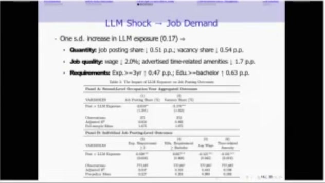
The headline slide is legible even though the table under it is not. After the shock, a one-standard-deviation rise in exposure goes with several changes. The occupation’s share of postings falls by 0.51 percentage points and its share of vacancies by 0.54 points. Posted wages fall by 2.0%. The probability that a posting advertises time-related amenities falls by 1.7 points. The share requiring three or more years’ experience rises by 0.47 points, and the share requiring a bachelor’s degree by 0.63 points (slide at 01:39:36). Fang turned the amenity number into “about 10%” of the 19% base (01:40:26). By our arithmetic, 1.7 over 19 is closer to 9%, so call it roughly a tenth.

The posting-share number is bigger than it looks. With 93 occupations the unweighted mean share is 100/93, or about 1.075%. A 0.51-point drop is then roughly 47% of the mean, by our arithmetic. Raymond’s slide independently says a one-s.d. increase “reduces posting share by about 48% of the pre-period mean” (slide at 01:59:35). That slide doesn’t give the denominator, so I will only say the two numbers are close. Either way this is a reallocation of shares in a fixed-size sample. It is not a 48% fall in the number of jobs, which is a point Raymond made at some length and which comes back below.

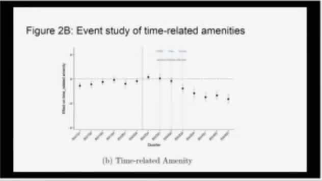
The dynamics tell Fang’s timing story. ChatGPT itself was never available in China. On the event-study plot the effects do not show up at the ChatGPT line. They show up after Chinese models launch: Baidu’s Ernie first, then Alibaba’s Qwen and ByteDance’s Doubao (01:41:36). Fang’s reading is that ChatGPT was “a jolt in the Chinese ai circle,” and then when domestic tools arrived “the labor market immediately responded” (01:42:45). Callbacks fall too. The slide says more human capital (five-plus years’ experience, a bachelor’s degree, an elite university) “partly mitigates the decline” (slide at 01:45:07).

The surprising part: seniority is paid in weekends

The best-known us result that Fang set this against is the “seniority-biased” story. Fang cited it to Hosseini, Maasoum and Lichtinger (2025): senior workers keep their jobs and their pay while junior positions disappear (slide at 01:26:18; 01:25:56). The China postings show a different pattern. When the authors split postings at three years’ required experience, the higher-requirement jobs show a slightly smaller wage decline. They also show a larger drop in advertised time amenities (slide at 01:43:10; 01:43:54). In Fang’s words, the more experienced “suffer also on the non-monetary margin.” So the pay of senior-looking jobs is partly protected, and the weekend is what gives.

It helps to be precise about what this observes. These are postings grouped by the experience they ask for. They are not employed seniors whose Saturdays were taken away. The outcome is whether a posting mentions weekends off, a five-day week or no overtime. Raymond’s slide said it directly: “zero does not mean the job lacks the amenity,” and the variable “measures advertised language, not realized working conditions.” But it is still an odd and informative pattern. If you care about wages the way labor economists usually measure them, you would see a senior segment that looks mostly fine. The damage is in a field that us postings don’t really have.

Fang’s explanation is legal. Chinese labor law, as Fang put it, protects “workers in their disputes with their employers … in terms of wages but not so much on non-wage benefits” (01:47:59). So the margin an employer can adjust cheaply is hours. The authors test a version of this. They split provinces by how often workers win labor disputes, and the slide says protection “may only buffer the wage dimension, not the hidden time amenity dimension” (slide at 01:47:57). I would not lean hard on it. Its wage “buffering” is the gap between an insignificant coefficient in high-protection provinces and a marginally significant one in low-protection provinces, with no test of the difference shown. Fang also called the mitigating effect “minor” (01:31:37). The legal story is Fang’s interpretation, and a plausible one. It is not a tested mechanism.

Applicants, and a null that gets a story

On the supply side, the regressor is the exposure of the applicant’s last occupation. The slide gives the average effect as “smaller than demand-side,” with juniors hit on callbacks and seniors and the highly educated hit on time amenities (slide at 01:46:58). The mobility table says applicants “slightly shift to low-exposure occupations, but only a little,” so “applicants are unlikely to fully offset the shock by themselves” (slide at 01:47:36).

Then there is the applied-wage result. There is “no statistically significant change in applied wages,” and the slide offers “a possible interpretation: applicants adjust wage expectations slowly” (slide at 01:47:02). In the talk this became “they are not adjusting … sufficiently” (01:47:18). That goes a step past the estimate. The outcome is the posted wage of the jobs people applied to. Posted wages in exposed occupations fell about 2% on average. So a null could also mean applicants moved toward jobs whose wages didn’t fall, which is the opposite of failing to adjust. That reading depends on some assumptions: that applicants target a similar mix of jobs, and that last-occupation exposure tracks the exposure of the jobs applied to. It also depends on the 2% being a real within-job wage cut rather than a change in which employers are posting. The confidence intervals are wide too. The null is a fact; the explanation is the authors’ guess.

Raymond: which shock, and which wage?

Raymond, who had read the draft, was generous and pointed. The sharpest point was about the variable the paper cares most about. “Weekends off,” Raymond argued, is not a non-wage amenity. Suppose one job says you’ll work Saturdays and another offers a five-day week for the same monthly pay. The first job’s effective hourly wage is lower (01:54:55). So the finding may be less “ai hits non-wage margins” and more “ai hits wages, measured properly.” The suggestion was to check what the posting language means in practice and then build an effective hourly wage from imputed hours. This doesn’t weaken the surprising result so much as translate it. If the advertised weekend tracks actual hours, senior-looking postings didn’t get a mild wage cut and a separate amenity cut. They got a bigger hourly wage cut, taken in a form that monthly-wage regressions miss. That would be a more uncomfortable paper, and probably a better one.

It is also worth looking at the pre-period on that plot, which is Raymond’s clean copy of the authors’ Figure 2B. The pre-period coefficients sit below zero and drift up toward the reference quarter before the post-launch fall. Fang’s slide says “no clear pre-trends.” The axis ticks aren’t readable, but the dots are not flat.

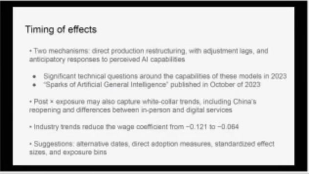
The second point was timing, and it is the one that should worry the authors. ChatGPT, released at the end of November 2022, was never available in China. The first domestic model was Baidu’s test launch in March 2023. So Raymond suggested defining Post by whichever domestic launch the authors think is the relevant shock (01:50:48). Then there is the calendar. In December 2022 China lifted its internal Covid mobility controls, and in January 2023 it reopened its borders (01:51:29). In-person activity came back at exactly the moment Post switches on, and in-person work is presumably what the exposure index calls unexposed. So Post × Exposure is also plausibly Post × Reopening, and the reopening would push in the same direction as the paper’s results. And in 2023, Raymond noted, nobody knew what these models could do. Firms would have had to be “very smart” to restructure production in anticipation, yet the wage event study shows effects starting “very early” (01:53:15).

The number to remember from the discussion is that adding industry-by-time controls cuts the posted-wage coefficient from −0.121 to −0.064. That is roughly a halving, by our arithmetic. The draft reports this in the appendix, and the authors did not show it in the talk. Raymond’s advice: “I might make that your main specification” (01:59:04). (The −0.121 is consistent with the 2% on Fang’s slide: multiplied by 0.169 it is about −2.0%, by our arithmetic.)

The third point was composition. A fixed 200,000 postings a year can measure shares, not quantities. If software postings fell in absolute terms while blue-collar service postings grew even faster, the software share could move for reasons unrelated to software (01:56:57). Callbacks have the same problem. If the volume of applications on the platform rises while job slots stay fixed, the callback rate falls “just mechanically” (01:57:10). Raymond also wanted the callback redefined as interview callbacks only, since the current measure bundles a phone call with a WeChat exchange. The closing suggestion was that the more direct ai effect on a platform like this may be screening. llm-written applications flood firms and break the signals they relied on, possibly before anyone restructures production (01:59:45).

The room, and Fang’s concession

The Q&A mostly asked why China looks so different. One questioner, called on as “Hannah” (the name is from the captions), asked for a control for automation exposure. China has invested heavily in robots, and that exposure may be correlated with llm exposure. The same questioner asked whether an occupation is even the same job across regions (02:01:05). The next questioner noted that in us data employment has mostly risen, with only 22-to-25-year-olds in exposed occupations lagging, and asked, “why are they so different?” (02:01:45). Another said every paper they knew found ai roughly benign for labor, and asked whether this was the first to look at posting flows on a platform rather than ex-post outcomes (02:02:46). A fourth made the jobs-are-not-occupations point. Frey and Osborne’s frightening automation numbers shrank to about 9% once within-occupation task variation was allowed for. The posting text could measure exposure job by job, and us age effects might really be job-breadth effects (02:03:38).

Then came the question that mattered most. A questioner Fang later addressed as Kevin proposed a business-cycle story. Chinese firms are liquidity-constrained, China was in a downturn, and a firm spending on ai capital would say, in the questioner’s words, “I just don’t have the money” to hire as many workers. That story, the questioner said, fits “basically all the cuts of the data” (02:04:55). Someone else followed up asking for placebo occupations such as construction (02:05:39).

Fang’s answer did not fight this. On placebos, the platform is strong in manufacturing back-office jobs, and construction isn’t really on it (02:05:53). On the downturn: “I think Kevin is right that China is in a pretty big … macroeconomic downturn” (02:06:29). Fang said there were 320 million gig workers by June 2026. (The captions garble the share of the workforce that goes with it, so I won’t repeat it.) Then came the concession: “we try to control for the time fixed effect but again there could be occupation interacting with time macro trends that is not being captured by the time fixed effects alone, so we are not giving a very crystal clear answer what is causing this” (02:07:28). What the paper does, Fang said, is compare more- and less-exposed occupations. The jobs-versus-occupations point becomes the next paper, on how job descriptions and task bundles are being redesigned (02:07:57). The automation control, the redefined Post date, the effective hourly wage and the interview-only callback got no direct answer.

That is a respectable place to end up. The descriptive facts are good and new. In a large Chinese platform, postings in more exposed occupations shrank as a share after late 2022. Their posted wages and advertised weekends fell. And the more senior the posting, the more of the adjustment showed up in weekends rather than pay. Whether that is the llm, the reopening, or a downturn landing on white-collar work is, by the presenter’s own account, not settled. Raymond’s reframing may be the paper’s best idea: the weekend is part of the wage. If so, the finding that “wages barely moved for seniors” means that wages moved for seniors, in the column where nobody was looking.