Interpreting and Steering LLM Agents for Social Simulations

Jiayue Fan, Arul Murugan, Shreyas Krishnan and Abhishek Nagaraj (UC Berkeley Haas), “Interpreting and Steering LLM Agents for Social Simulations,” presented at the NBER conference on AI and Economic Measurement, Stanford, 7 May 2026; discussant Matthew O. Jackson (Stanford). Source note: there is no public draft. As of September 2026 the authors’ project page still says a preprint is coming. Everything below comes from the twenty-minute talk and from frames of the slides shown on the day, and is attributed that way throughout — to the presenter, or to a slide at a particular minute. The presenter is almost certainly Nagaraj (Jackson refers to “Abishek’s talk”), but the auto-captions mangle names, so I mostly just say “the presenter.”

You want a subject. Not a person. People are expensive, slow, and — in precisely the dimension your theory needs them to vary — unwilling. What you want is what your colleagues on the other side of campus have had for decades: a mouse, ordered from a catalog, engineered at the genetic level to carry exactly the condition you are studying. The talk opened on Schelling’s segregation model, which got macro patterns out of trivially simple agents, and then made the move that organizes everything after it: “neural nets kind of offer a lab rat for social scientists.” Followed immediately by the twist, which is the actually interesting part, since biologists “don’t just use vanilla mice.” A slide put the 2007 Nobel in Physiology or Medicine on screen — gene targeting in mice — to establish that the animal is a designed object, not a found one. So: “if I have a theoretical model about risk preferences, can I go and get a risky LLM and order one from one of the companies.” He then conceded, cheerfully, that this “is not going to be a very big business model for the foundation lab companies,” which means academics have to build the menu themselves. That is the paper. Or rather, since there isn’t one yet, that is the talk.

What “inside” means. A transformer carries a residual stream: a vector of activations, per token, per layer, read and rewritten on the way to the next token. Mechanistic interpretability bets that those vectors are legible. The presenter’s addition is that they might also be writable — “maybe I can not just read out that preference, but I can change the mat to a ball.” Two techniques were compared, plus the baseline everyone actually uses.

The first is a sparse autoencoder: unsupervised, expensive, general. You map the dense activation into a much wider space where individual dimensions tend to carry human-readable labels, then you turn one up. The steering step, transcribed from the method slide shown at 02:41:20 rather than from any paper, is

where $z$ is the sparse feature vector read out of layer $\ell$, $e_i$ is the direction of feature $i$, $\alpha_i$ is how hard you push it, and the second expression decodes the edited features back into an activation that the forward pass then continues from. The presenter said the model they use has about 65,000 such features, and that training one of these things can cost tens of thousands of dollars — both spoken figures, not slide figures. The consolation is that once trained it works for every task you ever run.

The second is a linear probe: supervised, cheap, single-purpose. You fit a linear readout of one labeled property, then inject that same direction back in. From the slide at 02:42:05,

where $w$ is the direction fit by ordinary least squares against your labels, and $\lambda$ is the strength of the nudge. That $\lambda$ is the dial, and it matters later. The slide carried its own caveat: probes reveal readable information, “not necessarily the full internal mechanism.”

The third is prompting — telling the model it is a risk-loving individual — and a slide showed the real code, forty agents in a loop, each handed traits like “descriptions of unconventional thinking, especially ’thinking outside the box.'”

The implementation slide, at 02:43:35, is unusually concrete for a talk this fast: orchestration through John Horton’s Expected Parrot framework; base model Llama-3.3-70B-Instruct, eighty layers; sparse-autoencoder interventions at layer 50, probe interventions at layer 48; a note that the probe pipeline was also replicated on Qwen-2-7B-Instruct, though no results for that replication were shown. The autoencoder itself is not theirs — they use a pre-trained Goodfire one sitting on top of Llama. And the model is open-weights for a reason he stated flatly: “you can’t use [closed-source models] for these kinds of techniques, you need to be able to look inside of the blackbox.” Which is a real fence around the whole agenda. The lab rat has to be one you are allowed to dissect, so it will generally not be the best rat available.

The lottery. Fifty tokens guaranteed, or a coin flip for some larger number. The switching point — the payoff at which the agent flips to the gamble — is the risk preference, and risk neutrality puts it at 100. Unsteered Llama, the presenter said, switches at about 120: mildly risk averse, roughly plausible, fine. Read the model’s internals at that moment and the top features have, in his words, “nothing to do with risk aversion” — they are about being presented with options and having to pick one. “Calculated risk-taking behavior and entrepreneurial mindset” is there, boxed in red on the slide, but sitting mid-table. Push that feature up and here is what happens.

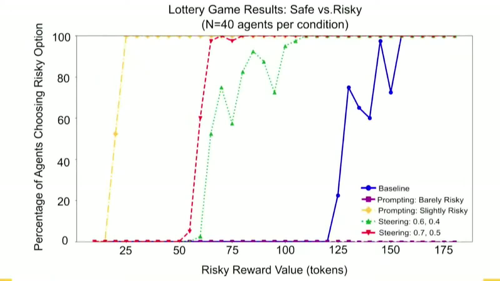
Forty agents per condition, per the slide title. The steered lines do move in the right direction and do land between the extremes, but they are wobbly and they cross each other, and the two settings are labeled with pairs of numbers that were never explained on the slide or from the podium, so I will not guess what they mean. The presenter’s own verdict is the honest one: “some variation but not precise control.” I should say that all the readings off that chart are eyeballed from plotted lines; the only printed thing on it is the axis.

The dial. For precision you need probes, and getting them costs something the presenter named out loud: “I’m going to throw away the generalizability or the general utility of SAEs” and engineer a classifier for this one task. What you get back is the prettiest object in the talk.

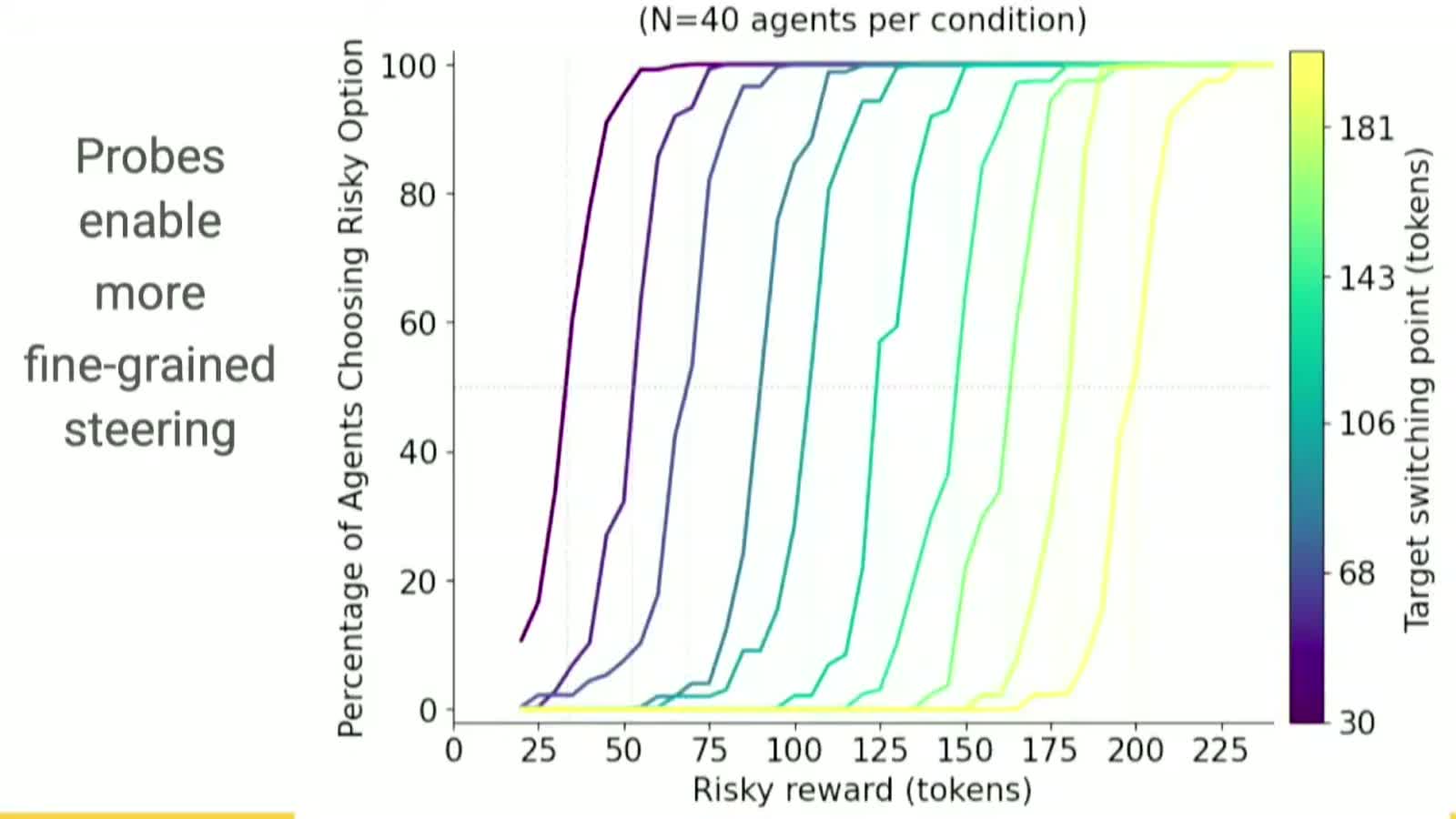
The colorbar is labeled “target switching point,” with printed ticks at 30, 68, 106, 143 and 181 tokens, and the curves cross fifty percent roughly where their color says they should. The colour is what you ordered; the curve is what arrived. The same trick was shown for the ultimatum game at 02:48:05, four curves, printed colorbar ticks at 30, 40, 50 and 60, with $\lambda$ named in the chart title as the thing being varied. He also asserted that the autoencoder found an altruism feature in the ultimatum game, but that slide was skipped, so it stands as a claim from the podium. And nowhere on either chart is there a calibration number — no reported gap between target and realized switching point, no error bars, no $R^2$. The claim is made by eye.

The thing that didn’t work. Two more tasks, both framed as capabilities rather than preferences: list uses for a brick, and improve a stapler. A second model, GPT-5, scored the answers one to ten on fluency, flexibility, originality and elaboration, with a footnote on the slide noting that the model is therefore not grading itself. The results slide is titled, by the authors, “SAEs unable to generate much change.”

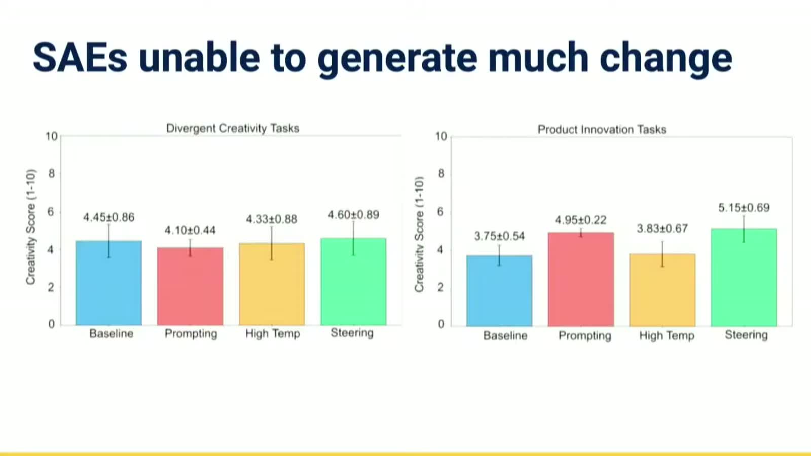
These eight numbers are printed on the slide and are the firmest evidence in the whole talk. On the brick, baseline scores 4.45 ± 0.86, prompting 4.10 ± 0.44, high-temperature sampling 4.33 ± 0.88, steering 4.60 ± 0.89 — everything inside everything else’s standard deviation, and prompting is the worst of the four. On the stapler, steering (5.15 ± 0.69) and prompting (4.95 ± 0.22) both beat baseline (3.75 ± 0.54), which is a real gap, but steering’s edge over just asking nicely is two tenths of a point. No test was shown for any of this, so none of it should be called significant. The presenter claimed probes did work on creativity, including out of sample, but showed no numbers and passed the slide in seconds; that is the least-evidenced claim of the twenty minutes and belongs in the piece only as a claim.

Where the surprise actually is. The stated punchline is that steering moves preferences and not capabilities — you can turn a dial on what the model wants, not on what it can do. That is clean and it is what the takeaway slide says. But look again at the first chart, because the more interesting failure there is the baseline’s, not the intervention’s. Prompting has two settings: “barely risky” leaves the agent at zero percent across the entire range, and “slightly risky” has it at a hundred percent by a payoff of 25, meaning it takes a coin flip for 25 over a guaranteed 50. Neither is a preference; both are a costume. And the unsteered model is no better behaved — roughly 75 percent risky at 130, 60 at 140, 98 at 145, 73 at 150. That is not a utility function, that is a staircase someone fell down. So what the probes actually buy is not more risk-taking. It is monotonicity: an agent whose behavior is a well-behaved function of the incentive, which is the minimum qualification for calling the thing an economic agent at all. Nobody said this from the podium, but it is what the chart shows.

Jackson. He discussed all three papers in one continuous set of remarks and spent about ninety seconds on this one, warmly. He picked the mouse metaphor back up and improved it: “we actually learn a lot about human disease by figuring out what kinds of lab rats did we have to build in order to test a medicine.” Which inverts the whole enterprise — the construction of the animal is itself the finding, and what you had to do to the model to make it behave is data about behavior. He treated the open-weights constraint as a feature rather than a tax, on the grounds that we will increasingly need “not just building better simulators, but understanding why they’re simulating in the ways that they are.” His one general warning was aimed at the room: LLMs are temporary, five years out we will be talking about something else, so extract lessons rather than facts about Llama 3.3. And then the 1980s, when minute-by-minute stock data arrived and the profession promptly discovered the day-of-the-week effect, the January effect, the index effect, the large-cap effect — “shiny new facts” — until “we have to start disciplining ourselves or we’re just going to be under a sea of potential research questions.” A feature space with 65,000 dimensions in it is, among other things, an industrial-scale shiny-fact generator.

His closer was the chess/Go paradox. Deep Blue was thirty years ago, AlphaGo ten, and these systems now make moves nobody can interpret. If a simulator predicts rain better, fine, take the rain. But “what if we start using it for predicting what’s going to happen to three different potential rate decisions by the Fed” and it cannot tell you why? His resolution named this paper’s tools: we will “need to be able to look under the hood eventually.” The authors did not answer, because there was no slot to — the chair went straight to open Q&A, and not one question in the general Q&A was put to this paper. Nobody asked about the wobbly curves, the missing calibration statistics, the GPT-5 judge, or whether forty agents per condition is enough. The chair, who is not named in the captions, did ask everyone about training-data contamination, and someone answered — probably this presenter, though the captions do not say — that in past work, on data they knew the model had been trained on, memorization rates ran maybe 10 to 20 percent, because “I don’t remember chapter six of a book I read in third grade.”

Anyway. The recipe the talk lands on is: use the autoencoders to discover what the model is using, and the probes to steer what you can define. Which is tidy, and also quietly circular, because the two halves don’t touch. The method that could tell you something you didn’t already know — that there is a feature in there about the Russian word for brick, say — is the one that produced the wobbly line and the flat bar chart. The method that produces the beautiful fan of curves is the one that, as he put it himself, is “completely useless for interpretation,” because you have to supply the labels and the target in advance. You order a mouse with the disease you specified, and the mouse arrives with the disease you specified, and it is genuinely useful to have it, but it has told you nothing about disease. There is a real tension here between finding out what is in the animal and building the animal you already drew, and the talk’s own evidence sits on both sides of it. Which is, to be fair, roughly where the mouse business started too.