Precautionary Sourcing and the Macroeconomics of De-Risking

Ester Faia, presented at the nber International Finance and Macroeconomics Program Meeting, 23 October 2026; discussant Doireann Fitzgerald. No public paper exists, so this note rests on the talk, the deck shown on screen and the deck posted on the nber agenda, and is flagged as such; the on-screen deck is taken as what the talk presented, posted-only numbers are marked, and the two disagree on the level of worker welfare.

You run an American manufacturer and you buy an input from China, because China makes it well and cheaply. You settle your recipe now and pay whatever the ingredients cost later. So you are holding a position in the input’s price, and like any position it has a mean and a covariance with your bad states. A diversified owner would worry only about the states that are bad for diversified owners. But suppose you cannot lay off your own risk. Then an input that gets dear exactly when you are in trouble is worth less to you than to the rival down the road with different troubles, at the same market price. A supply chain is a portfolio, held by somebody who cannot diversify.

Anyway, Faia’s claim is that this is what the retreat from China looks like. China’s share of us goods imports went from about 24% in 2017 to about 19% at the end of 2019, and it fell for goods with no Section 301 tariff as well as goods with one. Trade-policy uncertainty rose first. So: not “tariffs made China expensive” but “firms got nervous,” with the misallocation that implies, because you are now buying from Mexico “although Mexico is less efficient.” (Two small corrections to the talk. Faia said the tariffed series doesn’t go down; on the slide’s own chart it does, from about 21% to about 17%. And the slide says the share “falls before enactment,” but what the chart shows moving before enactment is the uncertainty index; both share series step down after the 2018Q3 line.)

The model

Start from Baqaee-Farhi (2019), make the input shares a choice as in Kopytov and coauthors (2024), and give each firm its own log kernel, $\lambda_i=\lambda^c+\xi_i$: the diversified owner’s kernel plus an uninsurable piece that is zero under complete markets. Firms commit shares, shocks land, and they buy quantities at realized prices. The lemma on slide 11 of the on-screen deck says the first stage is a very familiar object:

Here $\alpha_i$ is firm $i$’s vector of committed input shares, $a_i$ its log productivity in those shares (strictly concave), $p_j$ the log price of input $j$, and $\mathcal{R}_{ij}$ the input’s effective cost to that buyer. That is an asset-pricing formula with the sign turned around for something you buy rather than own. As Faia put it, the expected price is the same for everyone buying the input, “but how that input affects me depends only on me.” Slide 12 then takes the excess over the complete-markets valuation:

$\tau_{ij}$ is the risk-misallocation wedge, $\phi_i$ the degree of uninsurability, $\varepsilon_i$ the sector shock with covariance $\Sigma$, and $\mathcal{L}=(I-\alpha)^{-1}$ the Leontief inverse. The nice thing is that neither ingredient distorts alone. With a fixed network the kernel never touches the allocation. With complete markets every buyer has the same kernel and the endogenous network is efficient. You need links that move and risk that sticks, and then, with identical markups, risk by itself misallocates production. (The wedge is conditional in both directions. A buyer whom the supplier hedges has a negative covariance, as Faia said when asked, and a positive wedge lowers a share at an interior optimum without severing the link. This is not a model of universal flight.) Aggregated up, the wedges deliver what the deck calls a network-corrected Hulten (1978) loss, a quadratic form in the wedges. That is a paper-and-pencil result; the deck never puts a number on it.

The quantitative version has eight sectors and three origins, with origin shares chosen by logit. Two additions do the heavy lifting on the way to the data. First, a firm resets its origin shares with probability 0.4 a year, “a kind of Calvo not on the prices but on the shares,” which is how Faia finally matched the gradual decline after, in her telling, many months of failing to. Second, the kernel is endogenized. Workers are insured by a limited-commitment wage until the firm’s own participation constraint binds, at which point the firm says, more or less, “okay, guys,” and passes the shortfall into pay. So uninsurability is the complete-market kernel plus the multiplier on that constraint, calibrated on Guiso, Pistaferri and Schivardi (2005), and the wedge is positive for inputs that are expensive when workers’ real income is low. Capitalists are risk neutral and own the firms, which will matter shortly.

The evidence

The natural first move is a diff-in-diff on product-level shares, which finds a big retreat from China for products with and without tariffs, about 6 pp each in electronics and machinery, with Mexico and Vietnam gaining. The second is an event study on Panjiva firm-level imports, with the pre-shock China share as exposure. Exposed importers lose China share (slopes of −0.23 in 2018 and −0.21 in 2025, which are exposure slopes rather than average losses) and gain ally share. “When I first started to see the event studies I was very enthusiastic,” Faia said, and then she controlled for pre-trends: “Everything disappeared.” The slide is more exact: net of an exposure-specific linear trend, the break reverses sign.

Most people would stop there. Faia reads the pre-trends as anticipation, and builds a design around that reading. It is a firm-by-origin local projection on the Caldara et al. (2020) indices, orthogonalized to get a surprise and interacted with the firm’s 2015 to 2017 share from that origin, so identification comes from the shares.

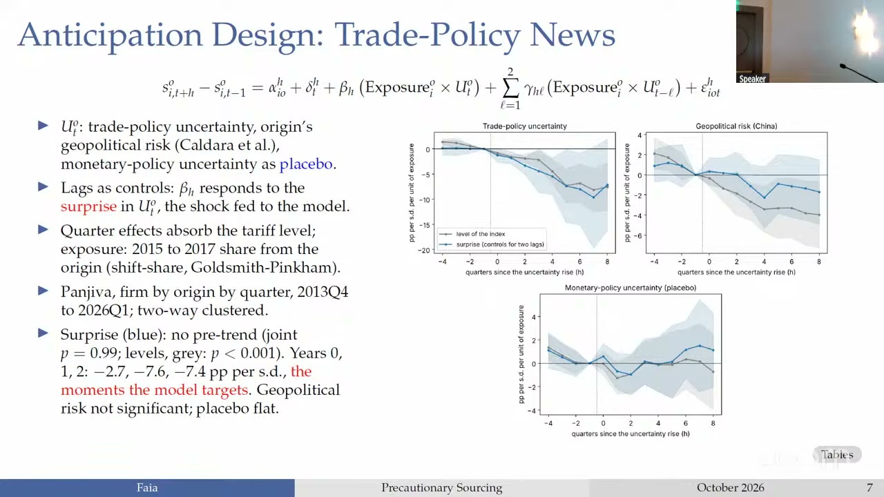
The surprise has no pre-trend (joint $p=0.99$, against $p<0.001$ for the raw index). The China share falls by −2.7, −7.6 and −7.4 pp in years 0, 1 and 2, per s.d. of the index and per unit of exposure, and both normalizations matter: these are not aggregate import-share changes. Geopolitical risk is not significant once orthogonalized (“it looked significant” before), the monetary placebo is flat, and across 7,000 firm-origin pairs and eight origins firms retreat from whatever origin they rely on.

It is a clever rescue, and three things are worth holding onto, none of them raised audibly in the room. A pre-trend alone does not separate anticipation from mean reversion, and an appendix page of the posted deck, never shown, names both: on a longer window the event-study coefficients for 2014 and 2015 are about as large as 2018’s, and firm China shares “mean-revert.” With one aggregate series, identification rests on those same shares. The slide’s “quarter effects absorb the tariff level” covers the common level but not exposure times a China-specific tariff change, which is how a China tariff reaches a China-exposed firm. And the plot stops at $h=8$, where the band runs from about −16 to +2, so the “year 2” moment cannot be read off the chart at all. Also, “the tariff level doesn’t do anything” was said aloud; the slide says only that the level effect does not survive pre-trends.

The surprising thing

The theory is about covariances. The numbers are not. The on-screen steady-state table is the key exhibit of the talk, and it is a pity that the audio is lost for the stretch when it was up.

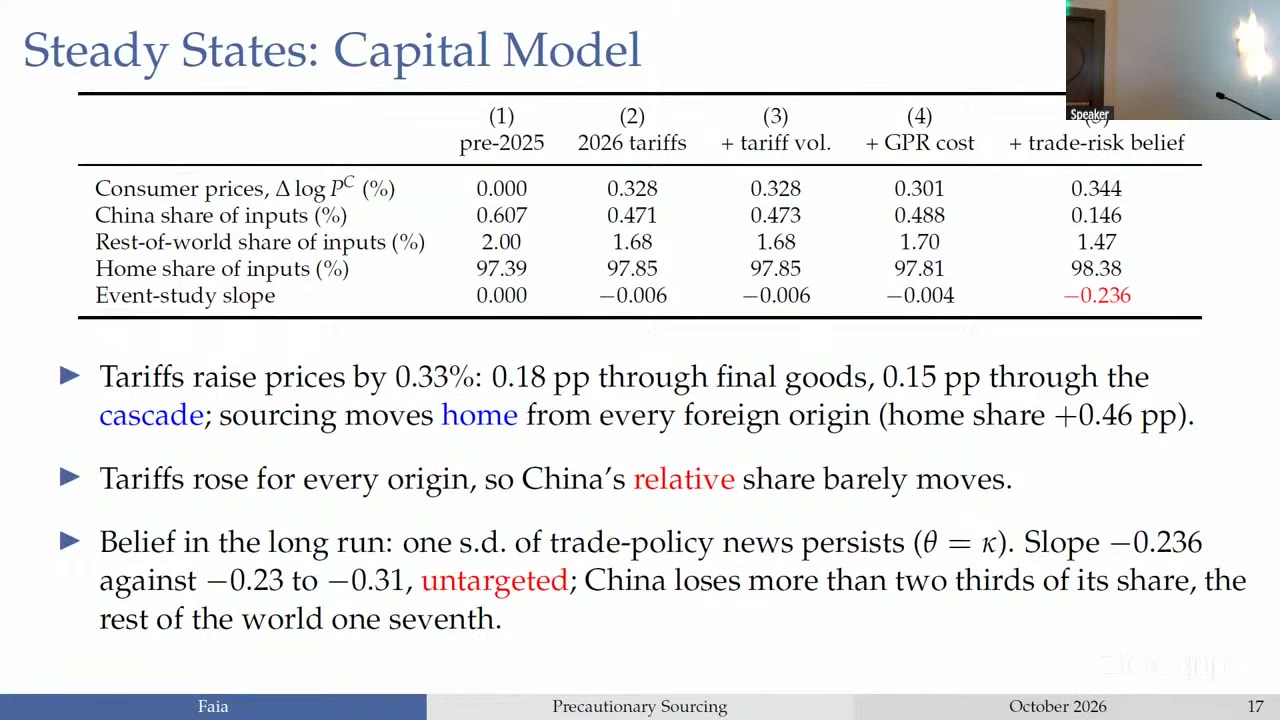
Run the 2026 tariffs through the model: consumer prices rise 0.33%, and the event-study slope is −0.006. Add tariff volatility, the thing the whole apparatus was built to price, and China’s share moves from 0.471 to 0.473, which is to say slightly up. (The column says only “+ tariff vol.” The natural reading is the roughly five-fold rise in the tariff-factor s.d. in the posted parameter table, but no slide ties them together.) Add geopolitical costs and little changes. Then add column 5, a “trade-risk belief” $\theta_t=\kappa\rho^t$, described as owners’ robust concern about the tariff process and placed directly on the risk-adjusted price of Chinese inputs, with a multiple of 0.184 on the rest of the world. China’s share falls from 0.488 to 0.146 and the slope goes to −0.236.

To be fair, nobody is hiding this. The posted deck says “the driver is owners’ beliefs about trade risk, not measured tariffs,” and Faia was plain about the general-equilibrium impulses: with the shock “only on the covariance” that pops up in misallocation, “I don’t go down very much”; with it “also on the investors’ kernel” she “managed to go down much more.”

Still, look at what the belief is. $\kappa=0.335$ and $\rho=0.70$ are, per the slide, the only parameters fitted to the anticipation design, and they hit its two moments, years 1 and 2. Since $\mathcal{R}$ is in log prices, $\kappa$ looks like a surcharge of about 33 log points on Chinese inputs, more than ten times the move in China’s tariff that the posted deck attributes to the same one s.d. of the index. (My arithmetic, assuming $\theta$ enters additively, which the slide implies without writing it out. Divide by the logit’s 0.25 and you get a log-odds hit of 1.34, against about 1.21 in column 5, so the magnitudes do line up.) The out-of-sample checks are two. Year 0 is missed, −5.7 against −2.7, on a posted page that seems to have been skipped on screen. The long-run slope is labelled “untargeted,” but it comes from holding one s.d. of news forever, and the slide does not say where −0.23 to −0.31 comes from. If that range is the event-study slopes, as I would guess, they are the ones that did not survive pre-trends. The gradualism, meanwhile, comes from the Calvo friction: without it the same belief sends the share down about 25 pp on impact in the posted plot.

Then there is the question of where the belief lives, which no slide answers. “Owners’ concern,” “the investors’ kernel” and risk-neutral capitalist owners all point to the diversified kernel $\lambda^c$, which is not $\xi_i$ and so not, by the theory’s own logic, the wedge. But a term added to $\mathcal{R}$ and not to $\mathcal{R}^{CM}$ is, by slide 12’s definition, a wedge. The first reading means the quantified retreat runs through the channel the theory treats as not distorting, and the deck’s opening question, is this efficient, has no quantified answer. The second means someone must explain why a firm-specific uninsurable concern is fitted to two aggregate moments. Without a paper this cannot be settled, so I will just note it as the first thing to ask.

Who pays

General equilibrium is where the dollar shows up. In steady state it appreciates about 4% on the tariffs, halving the price rise to 0.16%, and about 4% more with the belief. On impact in the impulse exercise it appreciates 1.3% (1.1% in the posted deck), consumer prices move at most −0.02% on a fixed basket, and net foreign assets end up 1.6% of gdp higher after two years. All of this, the concluding slide says, relies “on export market power and no retaliation.” So the tariffs are cheap for consumers on the assumption that nobody does anything about them.

Now the part where the two decks part ways, and the reader should know exactly how. The posted deck is dated about a week before the talk, and I follow the on-screen one, because the speaker’s words match it wherever the audio survives. On screen, workers lose 0.021% of consumption on average, and those at high-exposure metals and autos employers lose 0.308%.

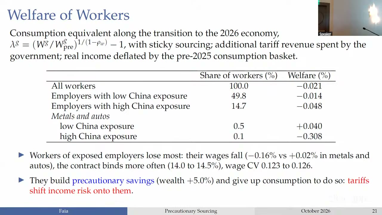
The posted deck’s headline was the opposite: “Workers gain about 0.5% of consumption,” and “Tariffs redistribute more than they destroy.” Part of that is the rebate, since the headline is the revenue-rebated column. But not all of it.

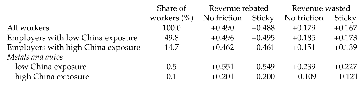
Compare like with like, sticky sourcing and revenue wasted. The posted column reads +0.167, +0.173, +0.139, +0.227, −0.121. The on-screen column reads −0.021, −0.014, −0.048, +0.040, −0.308. Every row is lower by 0.187 or 0.188. The cross-section is identical and only the level moved, and exposed workers’ wages tell the same story: they rise less in the posted deck (0.37% against 0.56%) and fall on screen (−0.16% against +0.02%). The on-screen slide adds two clauses the posted one lacks, “additional” revenue and income “deflated by the pre-2025 consumption basket,” so a change in the real-income accounting is the likely cause, but that is my guess and nothing in the sources says so. The takeaway is that the sign of the average worker’s welfare is a version-dependent accounting choice, while the ranking of groups is not. Faia said as much of the rebate: “if I give back the revenues to the workers actually there might be some gains but the distribution stays the same.” “They got a loss” is therefore conditional on the revenue being wasted. (And the −0.308 group is 0.1% of workers, as the table notes. The mechanism here is the contract binding slightly more often, 14.0% to 14.5%, and workers building precautionary wealth, up 5.0% on screen and 5.7% posted.)

What Fitzgerald pushed on

The recording is badly damaged here. Fitzgerald’s framing and first two comments survive only as slides, and the literature roundup and third comment are audible. There is no recorded Q&A and no recorded reply from Faia, so what follows stands unanswered. The in-talk exchanges survive only as Faia’s half of them.

The framing is deflationary. Any model in which choices made before shocks affect consumption possibilities after them will fit the facts, and the slide list of ones that do runs to sunk export costs, customer accumulation, buyer networks, inventories, and input networks chosen in advance. Fan and Luo and Bolívar are, in Fitzgerald’s words, “very close to your work.” Comment 1 asks whether it matters who chooses in advance: “Exporter-side mechanisms can certainly match tariff facts,” and “For efficiency, details matter.” So the sourcing retreat need not be an importer’s story, and the efficiency verdict depends on which story it is.

Comment 2 goes at the process: “Do tariffs really follow an ar(1) with normal innovations?” The slides show tariff histories that come in steps, including a China rate that goes from about 10% to a peak near 48% and back to about 22% in under two years. And then: “When we talk about ’tariff uncertainty’ increasing, are we confusing first and second moment shocks?” I think both land. The lemma’s “exact, not an approximation” rests on joint normality, and the posted deck’s table of shocks has the same index moving the level of China’s tariff as well as its volatility, so the local-projection coefficient is not a pure second-moment response.

Comment 3 is the one to think about. The standard assumption is that firms price states with the representative household’s marginal utility, and heterogeneous curvature across firms “is somehow less standard.” You can get incomplete insurance across countries without it, as in Bolívar, “so you don’t necessarily need to put it in at the firm level.” The discipline on firm-level risk pricing comes from “sort of a labor paper.” And the question: is firm heterogeneity important for the quantitative results, or would “something like in this Bolívar paper” be enough? The deck cannot say, because it reports no run without firm heterogeneity. What it does report is that the firm-level covariance channel, the one heterogeneity feeds, barely moves shares, while a belief fitted to two numbers does.

Which leaves a nice result and a nice question sitting slightly apart. The result, that the same supplier at the same price is dearer to the buyer whose bad states it correlates with, and that this misallocates only when links can move, is the thing to take away from the talk. The question is whether that is why anyone left China, or whether firms simply marked China up by something like 33 log points on a concern the deck does not locate, in which case the theory of who hedges what was doing rather less than the theory of what everybody believed.

References