Export Policy for Dual-Use Goods

Maxim Alekseev (HKUST) and Xinyue Lin (Harvard). Working paper dated 3 February 2026 from Alekseev’s site. Its first version carried the title “Trade Policy in the Shadow of Conflict: The Case of Dual-Use Goods”, which is how the presented papers on this list cite it. The PDF’s own footnote dates that first version 1 November 2025; the HBS working-paper page for it is dated October 2024 and the citing papers say 2024, so the footnote year is almost certainly a typo, but the document says what it says. No talk recording could be found; PDF-only digest. Figures and propositions are cropped from the PDF.

Export controls as a tariff problem with a second buyer

Export controls are the geoeconomic instrument with the least economic theory behind them. Sanctions have Becko’s optimal-tariff mapping; industrial policy has Kooi and GHL; export controls on chips, drones and machine tools have lists — the EU’s TARIC dual-use correlation table flags a growing number of HS6 categories, expanding with each deterioration in the security environment — and an intuition that one should not sell weapons to rivals. Alekseev and Lin give the lists a formula.

The set-up is deliberately ordinary. Take a two-country Armington trade model with a freely traded outside good that pins wages, so that the theory section is partial equilibrium. Then add one agent. A defence department collects lump-sum taxes from households, spends them on a non-traded military good, and the military good enters a contest with the rival’s. National welfare is household utility plus a weight on the contest. The government sets defence spending and export taxes at the same time, taking the rival’s spending as given. Everything in the paper follows from asking what a small export tax does to that objective (equation 21 at p. 10): it raises revenue, it raises the price the foreign military pays for its inputs, and it distorts domestic consumption. The middle term is the new one. The paper calls it a Marshallian externality: every unit a firm sells to the rival’s military lowers home welfare a little, and no firm prices that in, so the tax does.

The formula

With one exported good and no input-output links the optimal export tax is Proposition 1, equation 20 at p. 10.

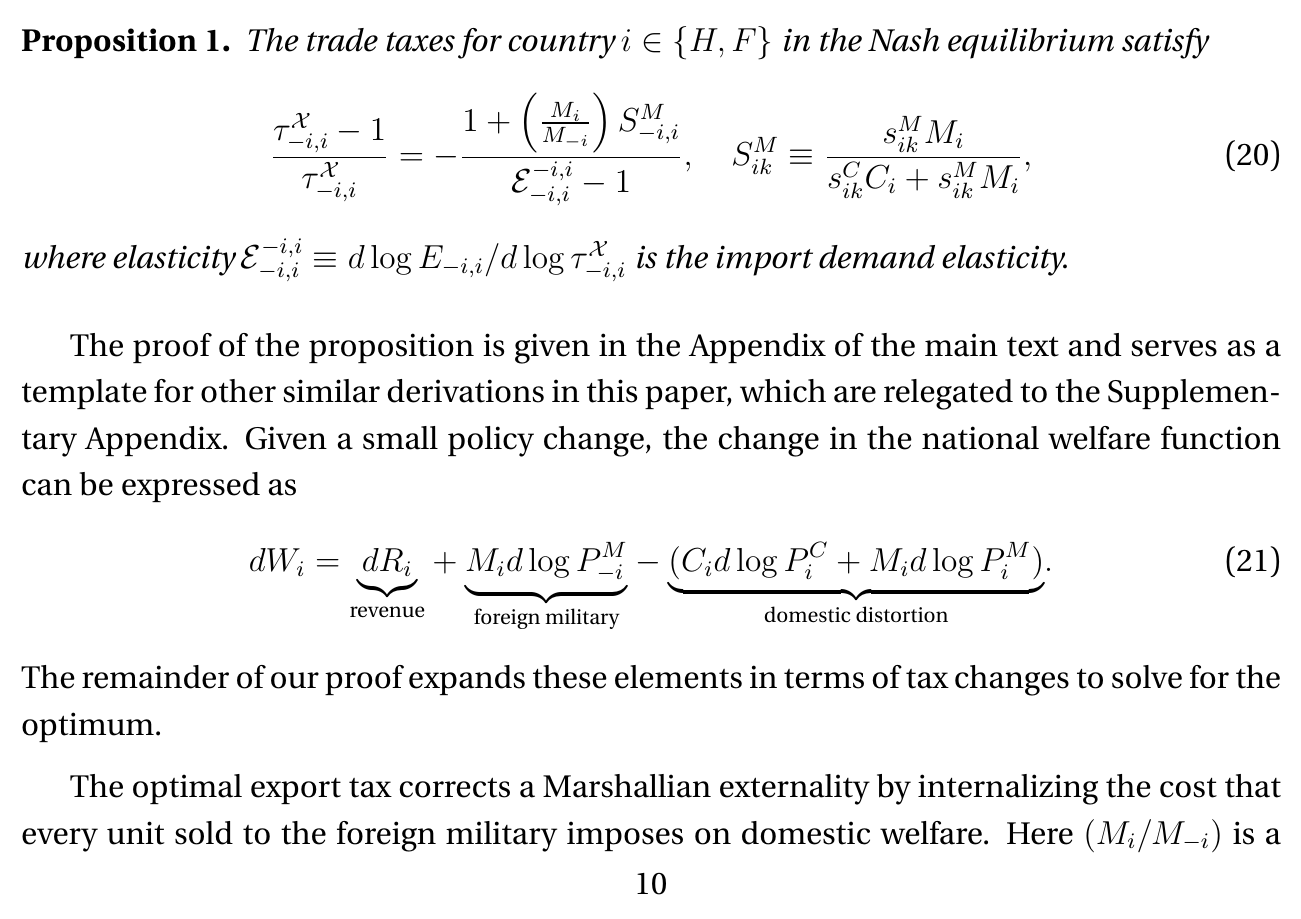
Here $\tau^{\mathcal{X}}$ is one plus the ad-valorem export tax, $S^M_{-i,i}$ is the share of the exported variety’s foreign sales that go to the foreign military, $M_i/M_{-i}$ is home military spending relative to the rival’s, and $\mathcal{E}$ is the import demand elasticity, which is negative, so the tax is positive. Set the military share to zero and you are left with $-1/(\mathcal{E}-1)$, the textbook terms-of-trade tax that extracts the monopoly markup. The military share is the correction, and the spending ratio is what scales it. Notice what is not there. The conflict weight $\beta_i$ never appears, because defence spending is chosen optimally and already absorbs it; the weight the government puts on winning enters only through how much it spends (p. 11). Notice also what the same logic says about imports: with constant returns and no market failure on the import side, the optimal tariff is zero — any domestic price manipulation is a deadweight loss (pp. 11 and 30). File that away.

With production networks the sales share becomes a centrality, and a second centrality appears to be subtracted from it. This is Proposition 2, equation 27 at p. 12, and it is the paper.

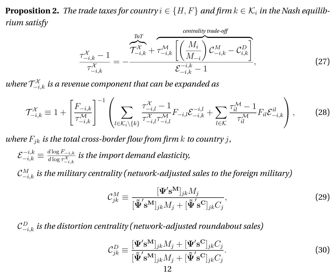
$$ \frac{\tau^{\mathcal{X}}{-i,k}-1}{\tau^{\mathcal{X}}{-i,k}} = -,\frac{\mathcal{T}^{\mathcal{X}}_{-i,k}

• \tau^{\mathcal{M}}{-i,k}\left[\left(\dfrac{M_i}{M{-i}}\right)\mathcal{C}^{M}{-i,k} - \mathcal{C}^{D}{i,k}\right]}{\mathcal{E}^{-i,k}_{-i,k}-1} $$

$\mathcal{T}^{\mathcal{X}}$ is a revenue component; the bracket is the trade-off. Military centrality $\mathcal{C}^M_{-i,k}$ is the share of firm $k$’s sales that ends up with the foreign military through every chain of intermediate use — the Leontief inverse applied to the military’s purchase shares — scaled, as before, by relative military spending. Distortion centrality $\mathcal{C}^D_{i,k}$ is the share that comes back to domestic final demand as roundabout imports: tax chip exports and the electronics Americans re-import get dearer. In an economy with no intermediate goods, military centrality collapses to the sales share and distortion centrality is zero, which is how Proposition 1 is the special case. The difference is divided by the elasticity, so the trade-off bites hardest for goods the rival cannot substitute. The paper’s illustration is chips, and the paper is careful to call the numbers hypothetical: imagine that of a dollar of US chip exports, thirty cents reach the Chinese military and twenty cents return in American electronics. Whether to tax then depends on how much the government spends on the contest relative to what its rival spends, and if China can make its own chips the elasticity is high and the tax should be low. Bans emerge as a second-best when instruments are coarse and the optimal tax is high enough. In general equilibrium (Proposition 3 at p. 19) the same trade-off reappears for factors — a factor-centrality term multiplied by the response of each factor’s price.

Military use, measured, predicts the lists

The formula’s sufficient statistics can be computed. The empirical measure is equation 31 at p. 14, $0 \le \mathcal{C}^M_{US,k}/\sigma_k \le 1$: military centrality in the closed US production network — 2018 BEA input-output tables plus Department of Defense procurement contracts, mapped from industries to HS6 goods — divided by Soderbery’s 2015 LIML import-demand elasticity, with the Broda–Weinstein and Fontagné elasticities as robustness. The closed US network is a deliberate choice. Observed cross-border sales already embody existing controls: US fighter-jet sales to China are zero in the data because they are banned, not because a fighter jet has no military use (p. 13), so a measure built on actual flows would tell you what is already controlled rather than what should be.

The top of the distribution is aluminium powders, warships, tanks, aircraft engine parts and shipbuilding components; the bottom is fresh food, tobacco, precious metals and cars (Table 1 at p. 16). Starting from no tax and equal military spending, the formula prescribes roughly 200 percent on aluminium powders and 40 percent on aircraft engine parts (p. 14). Some goods that score high are not on any list — drilling platforms, dredgers, tugs — which is either a gap in the lists or a reminder that the measure is a closed-economy sales share and not a threat assessment.

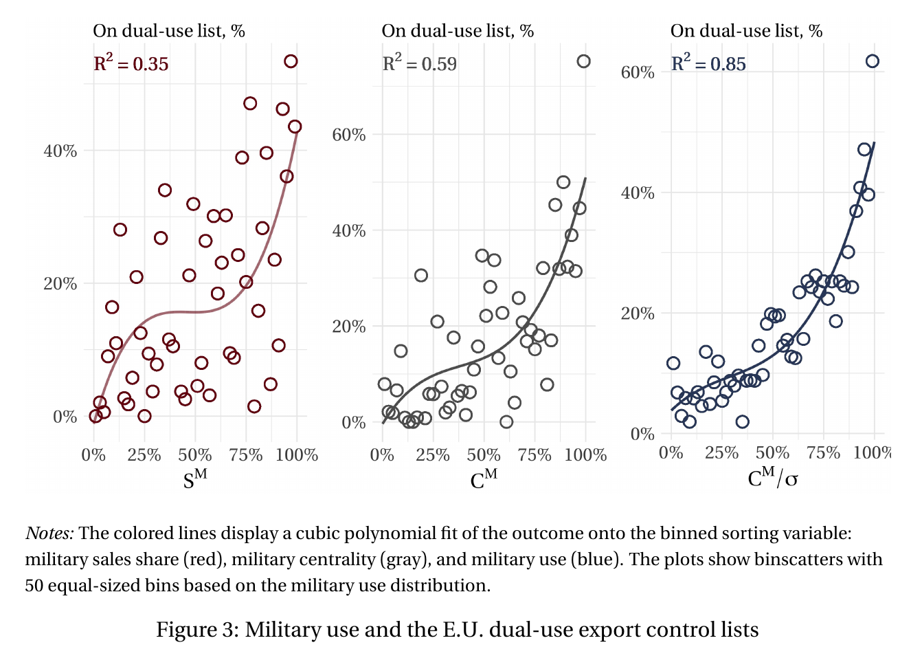
Checked against the 2018 EU dual-use list, moving from the bottom to the top of the measure raises the probability of being listed from 5 to 50 percent, and a cubic in the measure fits with an $R^2$ of 0.85 against 0.35 for the raw military sales share and 0.59 for centrality without the elasticity scaling. One caution on that number: it is a cubic fitted to fifty bins. At the good level, across 5,135 HS6 codes, the measure alone explains about 0.06 of the variance in list membership against 0.02 for the sales share (Table B.4 at p. 36); the ordering survives, the level does not. What the comparison does establish is that both the network propagation and the substitutability carry decision-relevant variation. The measure also predicts the US BIS restrictions imposed after 2022, and Global Trade Alert’s export non-tariff measures announced between 2018 and 2022 shift steadily toward high military-use goods (Figures B.4 and B.5). Existing export-control practice looks like an approximation of the model’s rule, arrived at without the model.

How much can export policy do

The quantitative section moves to general equilibrium with factors in fixed supply, adds Chinese input-output tables, and calibrates a US–China contest with a passive rest of the world. One assumption does a lot of work: the military procures from domestic industries only, and imports reach it only through the network (p. 20). The weight on the contest is backed out by revealed preference — a marginal tax dollar to the military must be worth a marginal dollar to households — and the headline is about 2.5 times annual US GDP. That is the last column of Table 3 at p. 23, which counts stockpiles and allies’ budgets and stockpiles as part of the prize; with the yearly budget alone it is 0.36 times GDP, and China’s figure in the headline column is 1.39 times US GDP. The returns to scale in military units, $\gamma \approx 0.5$, come from a GMM on Western-bloc spending as a best response to Eastern-bloc spending over 1950 to 2021, using the Soviet collapse as the instrument; the intuition is that US spending fell less than one-for-one when the Eastern Bloc’s did.

 and the foreign-to-home consumption ratio (horizontal), for the baseline export tax, no stockpiles, smuggling through third countries, coalition enforcement, and an import tax instead; each segment runs from the unilateral weight to a universalist one.’)

The counterfactuals are sober. China’s unilateral export policy shifts the military balance by 2.1 percent against 1.7 for the US, and the US overtakes China only when export enforcement is coordinated with the Western coalition, at which point its impact is three times China’s. Depleted stockpiles double the impact of trade policy; rerouting through third countries cuts it by more than half. Welfare effects are small — plus 0.2 percent for the US, plus 1.5 percent for China (Table C.1). And here is the reversal you filed away. In partial equilibrium the optimal import tariff was zero. In the calibrated model import tariffs are the United States’ most effective unilateral instrument, a little over 3 percent on the military balance read off Figure 4, because with factors in fixed supply a tariff shrinks China’s entire budget, and the military is bought out of that budget (p. 23). Export controls work on the price margin of a basket that is mostly domestic; tariffs work on the income margin of the whole economy. The paper’s summary is that roundabout network targeting has modest pass-through because militaries run on domestic resources — true in the data, and also partly what the calibration assumed.

Where it sits

This is the paper that fills the export-control gap in 1.4, which until now had the chokepoints (Digital Chokepoints), the innovation response (Flynn et al.) and the resources (critical minerals) but no theory of the instrument itself. It uses Baqaee–Farhi’s network machinery and Becko’s optimal-tax logic, and its military-use measure is a data product in the same family as Liu–Yang’s power measure and CMS’s power statistic. Read it with Export Sanctions (Egorov et al.), which measures what Russian export controls did to output, and with Geoeconomic Pressure, which finds that firms hit by export controls respond with R&D. That is the elasticity rising over time, which the formula puts in the denominator and the counterfactuals put in the smuggling line — the lists, it turns out, were already asking whether the rival can make it themselves, which is the same question that tells you how little the list will do.