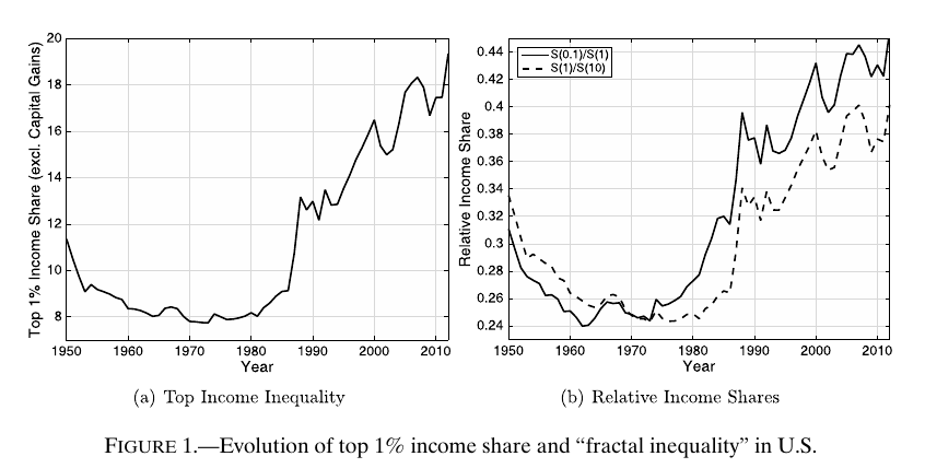
1 What?
The main contributions of this paper are: first, to show that the most common framework (a simple Gibrat’s law for income dynamics) cannot explain rapid changes in tail inequality, and second, to suggest parsimonious deviations from the basic model that can explain such changes.
2 Why?
2.1 Income inequality as per the power law

A large theoretical literature builds on random growth processes to theorize about the upper tails of income and wealth distributions. Early theories of the income distribution include Champernowne (1953) and Simon (1955), with more recent contributions by Nirei (2009), Toda and Walsh (2015), Kim (2015), Jones and Kim (2014), and Luttmer (2015). Similarly, random growth theories of the wealth distribution include Wold and Whittle (1957) and, more recently, Benhabib, Bisin, and Zhu (2011, 2015, 2016), Jones (2015), and Acemoglu and Robinson (2015). All of these papers focus on the income or wealth distribution at a given point in time by studying stationary distributions, and none of them analyze transition dynamics.
3 How?
Math: employed tools from ergodic theory and the theory of partial differential equations.
3.1 The standard growth model
3.1.1 Income dynamics
Time is continuous, and there is a continuum of workers indexed by \(i\). The dynamics is expressed using the dynamics of logged income \(x_{it} = log w_{it}\): \[ dx_{it} = \mu d_{t} + \sigma dZ_{it} + g_{it}dN_{it} \] where:
- \(Z_{it}\) is a Brownian motion
- \(N_{it}\) is a jump process with intensity \(\phi\)
- \(g_{it} \sim f(.)\)
Assumption: \(\mu\), \(\sigma\), and \(f(.)\) do not depends on time (Gibrat’s law)
This dynamics can be considered as a special case of “permanent-transitory model” of income dynamics, but without the transitory parts.
3.1.2 Stationary income distribution
Following a Pareto distribution: \[ \mathbb{P}(w_{it}> w) \sim C w^{-\zeta} \]
The constant \(\zeta\) is called the “power law exponent”, a smaller \(\zeta\) corresponds to a flatter tails. \(\zeta\) is a simple function of \(\mu\), \(\sigma\), and \(f(.)\). Without jump process \(\phi = 0\): \[ \frac{\sigma^{2}}{2} \zeta^{2} + \zeta \mu - \delta = 0 \]
TODO 3.2 The augmented random growth model
4 And?
4.1 For the standard growth model
- An increase in the variance in the permanent component of income \(\sigma^{2}\) in the standard random growth model is not a promising candidate for explaining the observed increase in top income inequality.
- It is also worth emphasizing again that allowing for jumps (\(\phi\) > 0) in the income process would only slow down the speed of convergence even more.
This post is in the collection of my public reading notes.