1 What?
2 Why?
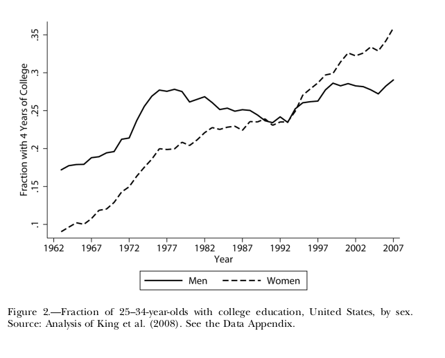
Figure 1: Increasing rates 25-34-year-olds woman with 4 years of college education
Past studies focused on changes in average costs and benefits of education for men and women over time -> They implicitly relied on a model of indiviual choice. (Jacob 2002; Buchmann and DiPrete 2006; DiPrete and Buchmann 2006; Goldin, Katz, and Kuziemko 2006)
3 How?
3.1 Optimal investment in colleage education by an individual
3.1.1 Model specifications
Consider the optimal investment in college education by different individuals: \[ S = F(h, H, A_{c}, A_{n}) \] where:
- \(h\) is time spent at college
- \(H\) measure the stock of human capital prior to any investment in \(S\)
- \(A_{c}\) and \(A_{n}\) measure cognitive and non-cognitive skills
Assumption: \(F_{h}\), \(F_{H}\), \(F_{c}\), \(F_{n}\) is positive; \(F_{hh} < 0\).
Target function: the disctounted expected utility: \[ V = U_{1}(x_{1}, l_{1}, H) + p(S; H)\beta U_{2}(x_{2}, l_{2}, S; H) \]
- \(\beta\): discount rate
- \(p\): prob. of surviving to the end of the next period
- \(x\): consumption of goods
- \(l\): household time
Assumtion: Utility is increasing and concave in \(x\), \(l\), \(S\).
There is also the assumption of full annuity insurance – which implies that expected disctounted consumption is equal to expected discounted income. Then, the full wealth budget constraint over the two periods is written as: \[ x_{1} + \frac{px_{2}}{1 + r} + w_{1}l_{1} + \frac{pw_{2}(S, H)l_{2}}{1 + r} + T(h) + w_{1}h = \\\ w_{1} + \frac{pw_{2}(S, H)}{1 + r} + \frac{pM(S)}{1 + r} = W \]
- \(r\): fixed interest rate
- \(W\): expected full wealth
- \(w\): hourly earnings
- Total time in each period is normalized to one
- \(T\): tuition and fees
- \(w_{l}h\) the earning forgone from being incollege
- \(M(S)\): gain from marriage in the second period, which is increment to expected wealth, and \(M_{s} > 0\).
Assumption: \(w_{2}>0\) (education should raise hourly earnings)
3.1.2 Solving strategy
Here I summarize the solving strategy sufficiently enough only to highlight interesting mechanisms.
Find \(S\), \(H\) that maximizes \(V\) under thee budget constraint.
- The first-order condition (foc) for consumption \(x\):
\[ U_{1x} = \mu \text{ and } p\beta{}U_{2x} = \frac{\mu{}p}{1+r} \] under full annuity insurance, uncertainty is not taken into the model, so: \[ \beta U_{2x} = \frac{U_{1x}}{1 + r} \]
- The foc for time spent in the household \(l\):
\[ U_{1l} = \mu w_{1} \text{ and } p\beta U_{2l} = \frac{\mu pw_{2}}{1 + r} \]
- Use \(e_{2}\) to denote the hours worked in the second period. The focs for the optimal time spent in college, divide both sides by \(\mu\) and \(F_{h}\), is given by: \[ \frac{pe_{2}w_{2s}}{1 +r} + \frac{\beta p_{s}U_{2}}{U_{1x}} + \frac{p_{s}(e_{2}w_{2} - x_{2})}{1+r} + \frac{pM_{s} + p_{s}M}{1 +r} + \frac{p\beta U_{2s}}{U_{1x}} = \frac{w_{1} + T_{h}}{F_{h}} \]
Let’s delve into individual terms in the last equation:
- \(\frac{pe_{2}w_{2s}}{1+r}\)
- the discounted expected increase in earnings from greater college education. This is the term that dominate discussion of “rates of return” to education in education literature.
- \(\frac{\beta p_{s} U_{2}}{U_{1x}} = \frac{p_{s}\beta U_{2}}{\beta(1+r)U_{2x}} = \frac{p_{s} U_{2}}{U_{2x}(1+r)}\)
- The second term measures the utilities gained on the probability of surviving in the future. \(\frac{U_{2}}{U_{2x}(1+r)}\) is called “the statistical value of life”, estimated to be in \$3-\$7 for a young male in the us.
- \(\frac{p_{s}(e_{2}w_{2} - x_{2})}{1+r}\)
- The benefit from an increased probability of survival in the future if future earning exceed education.
3.2 Market for college graduates
4 And?
Main takeaways:
Elasticity of supply of women and men to college depends on the amount of heterogeneity across women and across men in the cost of attending college.
- If women have a higher elasticity of supply to college, then even for equal changes in the benefits of college for men and women, women can overtake men in college attainment.
Women on average find school less difficult than men -> Increase the net benefit of college
Inequality of total cost of education appears to be lower among women than men. -> Women supply to college was more elastic than men -> When demand for college graduates grown, more women responded in increasing college attention.
This post is in the collection of my public reading notes.