Dollar Dominance and the Transmission of Monetary Policy

Michael McLeay (Bank of England) and Silvana Tenreyro (LSE), “Dollar Dominance and the Transmission of Monetary Policy,” Quarterly Journal of Economics 141(1) (2026), 605–666; advance access 22 September 2025, editors Robert Barro and Nathan Nunn, open access. Presented by Tenreyro as the 47th Barcelona School of Economics Lecture, Institut d’Estudis Catalans, 11 October 2024, sponsored by Banc Sabadell and introduced by Jordi Galí; there was no discussant, and about twenty-two minutes of Q&A followed. All page numbers below are journal pages of the published version. The images are tables and figures cropped from the published version, plus one frame from the talk, as each caption says.

The inference

Here is a fact about the world, and here is an inference that has been drawn from it. The fact: most international trade is invoiced in US dollars, even when the United States is not involved. Tenreyro opened the talk with the country-by-country version, which does not appear in the published paper: Spain sends under 5% of its exports to America but invoices over 30% of them in dollars; Argentina and Brazil invoice over 90% in dollars against a US export share under 20%; and while trade with the United States is less than a tenth of world trade, more than half of all trade is priced in dollars [00:08:30–00:09:36]. This is dollar dominance, and it is true, and it was documented carefully by Goldberg and Tille, by Gopinath and co-authors, and by others over the last fifteen years.

The inference: if your exports are priced in dollars, then when your currency depreciates, the dollar price of your exports does not fall, so foreigners do not buy more of them, so the exchange rate no longer does the thing Milton Friedman and Mundell-Fleming said it did. Expenditure switching is dead. A flexible exchange rate is no longer an automatic stabilizer, so your independent monetary policy is worth less than you thought, and the IMF’s 2019 external sector report duly suggested that countries in this position may want other tools — capital controls, macroprudential measures — to do the job the exchange rate can’t. This is the “dominant currency paradigm,” and if you are a central bank in an emerging market it has been telling you, fairly directly, that you are less powerful than your predecessors.

McLeay and Tenreyro’s paper is about the gap between the fact and the inference. The inference needs two more assumptions that the fact does not supply. It needs the dollar-invoicing exporter to have monopoly power, so that there’s a downward-sloping demand curve to be stuck on. And — this is the load-bearing one — it needs the dollar price to be sticky: unable to move for a year or so after the exchange rate does. Stick those two assumptions in a model, depreciate the peso, and nothing happens to exports. Cost in dollars falls, price in dollars doesn’t move, quantity demanded doesn’t move, the exporter pockets a fatter margin and goes home.

Who prices in dollars

Now ask who actually prices in dollars. The paper’s answer, built from three empirical observations, is: the people least likely to satisfy either assumption. Homogeneous goods — things traded on organized exchanges or against reference prices, in Rauch’s classification — are over 70% of developing-country exports, around 60% of emerging-market exports, and about 35% even for advanced economies (Chile at around 86% and Ghana at 85% sit well above that, with Norway at 76% and Russia at 73%). Homogeneous goods have flexible prices: Nakamura and Steinsson’s median monthly frequency of price change is 10.8% for finished producer goods and 98.9% for crude materials, and commodity prices change by the second. And homogeneous goods are precisely the ones invoiced in dollars. Across a panel of countries, a 10-point rise in the homogeneous share of exports goes with a 7-to-8-point rise in the dollar-invoiced share.

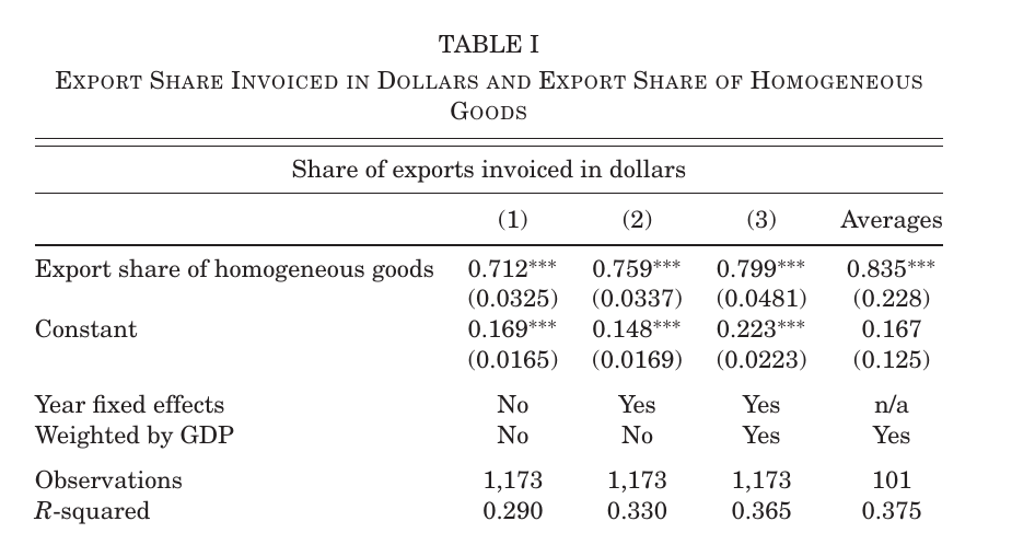
The third fact has a logic that goes back to McKinnon in the 1970s and Magee and Rao in 1980: you use a vehicle currency because you are a price-taker in a competitive market and need to keep your price continuously comparable with everyone else’s. Dollar invoicing, on this reading, is a symptom of price flexibility, not of price rigidity. The dominant currency literature took the same observation and inferred the opposite.

So why did anyone believe the prices were sticky? Because of pass-through regressions. Depreciate the peso by 10%, look at the dollar price of Argentine exports, and it barely moves. “Limited exchange-rate pass-through,” it was called, and it was read as evidence of a nominal friction.

Three pictures

The paper’s Section II is three supply-and-demand diagrams, and Tenreyro spent the first third of her lecture on them, because they are the whole argument. In all three, a depreciation shifts the exporter’s marginal-cost curve down when expressed in dollars, since some input costs (wages, rents, non-tradables) are sticky in pesos.

Picture one is the monopolist with a sticky dollar price. Cost falls, price can’t move, quantity doesn’t move. This is the dominant currency paradigm.

Picture two is a perfectly competitive commodity exporter. Demand is a horizontal line at the world price. Cost falls; the price also doesn’t move — but not because of any friction, because the exporter faces an infinitely elastic demand and could not move the world copper price if she tried. Instead she slides down her marginal-cost curve and sells more, until her rising marginal cost has eaten the whole depreciation. Zero pass-through, large quantity response. The observable price behavior is identical to picture one; the implication for exports is the opposite.

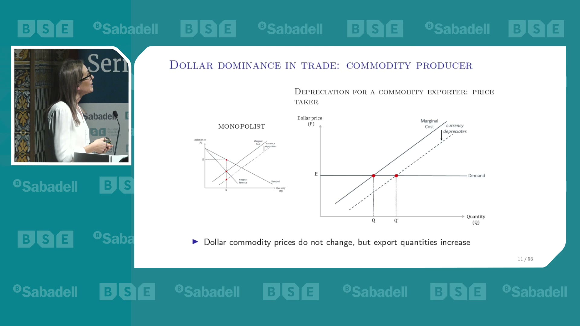
Picture three is the intermediate case, which is the one the model actually uses: a monopolistically competitive exporter facing a very elastic (but not flat) demand, with flexible prices. Here the exporter does lower her dollar price — fully, optimally, by as much as she wants to — but because demand is so elastic, the optimal price cut is tiny and the quantity gain is large. Low measured pass-through is an equilibrium outcome: the firm passes through every cent of its marginal-cost change, but the marginal cost rises as it expands, and the demand curve is so flat that the price barely has to move to clear a big increase in sales.

The point Tenreyro hammered, in the talk and in the paper, is that a pass-through regression cannot distinguish these cases. “Just observing lack of pass-through is not telling us whether the price is sticky, there’s a nominal rigidity, or simply there’s high elasticities of demand and the producers are price takers.” Reduced-form pass-through regressions omit marginal cost, and in a world where marginal cost moves to offset the exchange rate, they will attribute the offset to stickiness. The whole normative edifice was built on an identification failure.

The model and the headline number

The formal version is a small-open-economy New Keynesian model with a twist in the nesting. Standard international-finance models put the elasticity of substitution between countries’ baskets at the outer layer and allow no competition at a lower level; this one, following Feenstra and the trade literature, puts sectors outside and lets varieties from home and abroad compete within a sector. That lets you have a low cross-sector elasticity (2, from Gopinath et al.) alongside a very high within-sector elasticity for the export good (17, Broda and Weinstein’s estimate for crude oil, which happens also to be their mean across all products at the finest disaggregation). Exports are priced in dollars and fully flexible; wages, non-tradables and imported differentiated goods are Calvo-sticky with four-quarter durations, which is where monetary non-neutrality comes from. Export production has mildly decreasing returns to scale (0.85, backed out of the structures share of Canadian mining value added), which is the supply constraint. Incomplete markets, a Taylor rule, a 100bp monetary shock that after endogenous policy response cuts the rate by about 25bp and depreciates the currency by about 0.5%. The authors call it “mixed currency pricing,” MCP, because it nests the sticky-dollar-price DCP model and the Mundell-Fleming PCP model as parameter restrictions.

The equation the whole result rides on is the export demand each home variety faces from the US (equation (36), p. 633; the rest-of-world demand is the same with different subscripts):

Here $Y^{g_H}_{HU,t}(\omega)$ is US demand for home variety $\omega$ of the export good, $P^{\text{USD},g_H}_{HU,t}(\omega)$ is its dollar price relative to the dollar price index of that good in the US, $P^{\text{USD}}_{U,t}(g_H)$, $|\Omega^{g_H}_H|$ is the number of home varieties, $\gamma^{g_H}_{HU}$ is the US preference weight on home’s varieties, and $C_{U,t}+X_{U,t}$ is US final plus intermediate demand. The only thing that differs between the models is the exponent: with $\eta_{g_H}=2$ a 1% price cut buys 2% more sales, with $\eta_{g_H}=17$ it buys 17%, which is why a price cut too small to see in a pass-through regression can move export volumes by a percentage point.

Table III, on p. 639, is the paper in five rows. Same 0.52% depreciation in all three models. Under producer-currency pricing (Mundell-Fleming) the dollar export price falls 0.34% and export quantity rises 0.69%. Under dominant-currency pricing the price falls 0.07% and quantity rises 0.14% — the channel is off. Under MCP the price falls 0.06%, indistinguishable from DCP, and quantity rises 0.95%, more than Mundell-Fleming. Output rises 0.81% versus 0.42% under PCP and 0.32% under DCP. On impact the gap is starker still: export quantity rises 0.96% under producer-currency pricing and 1.34% under MCP (p. 638). The model reproduces the price facts that motivated the dominant-currency paradigm and discards its policy conclusion in the same table.

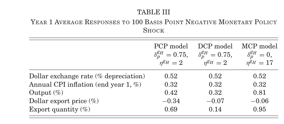
Her own summary of that table, in the talk, was that “we can restore the price properties of the dominant currency literature but allowing for the quantity responses” [00:35:16].

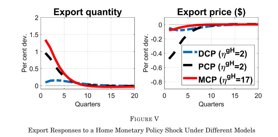
What limits the expansion is supply, not demand. Figure VIII varies returns to scale: with constant returns the export boom is very large; with steep marginal cost it is small. Tenreyro was candid that this is the parameter they know least about, and that it will differ by country and by commodity — pumping more oil is not the same as planting more soybeans — which is part of why the paper does the Canada and Chile calibrations separately. The other offset is wage inflation: with sticky wages it is small, but as wages become more flexible the depreciation buys less, and at fully flexible wages and prices it buys nothing. You still need some nominal friction somewhere in the cost base for monetary policy to work. The paper just moves it from the export price, where the evidence says it isn’t, to wages and non-tradables, where the evidence says it is. (There is a nice footnote linking this to Barro and Tenreyro 2006: what matters is the wedge between marked-up and competitive prices, not which layer of the production chain is sticky.)

Advanced economies get a section too. Add a second export sector that is differentiated and sticky in producer currency, vary its share between 20% and 80%, and aggregate exports respond about the same either way, because the PCP firms expand through the Friedman channel (big price cut, low elasticity) and the flexible dollar-pricing firms expand through the MCP channel (tiny price cut, high elasticity). In the Q&A the audience pressed on exactly this — if the UK also shows the “conventional” result, which countries is the paradigm supposed to describe? — and Tenreyro’s answer was that differentiated-goods exporters like the US and UK are basically Mundell-Fleming, commodity-heavy emerging markets are MCP, and the conclusion “the exchange rate is an automatic stabilizer” holds in both; the only thing being argued against is the recent literature’s claim that it doesn’t.

The evidence

Since prices can’t tell the models apart, the paper tests quantities. It is honest about how hard this is: exchange rates are endogenous, commodity-price shocks dominate their variation and produce a positive unconditional correlation between appreciation and exports (copper goes up, the peso goes up, Chile exports more copper), and monetary shocks are small and getting smaller. There’s a simulation exercise showing that even an econometrician handed the true monetary shock series and running a VAR on model-generated data recovers the impact responses but struggles with the dynamics, and gets very imprecise once shock variance drops to its post-2000 level.

With that caveat, three exercises. First, local projections on a panel of 37 emerging and developing economies, using Brandão-Marques et al.’s monetary shocks (residuals from a forecast-augmented Taylor rule). A tightening that raises the policy rate by one point appreciates the currency by 0.3–0.6%, and dollar exports fall by an average of 0.99% over the first year, peaking at over 1.5% after eleven months. The model said 0.95%. Industrial production falls too. The sticky-dollar-price prediction of roughly no export response is not what the data show.

The regression behind that figure is a Jordà local projection with country fixed effects (equation (39), p. 651):

$z_{i,t+h}$ is the outcome (log exports, CPI, industrial production, exchange rate) in country $i$ at horizon $h$ months; $\hat\epsilon_{i,t}$ is the monetary shock, the residual from a forecast-augmented Taylor rule (eq. 38) that purges past inflation, output growth, exchange-rate changes and the central bank’s own 12-month-ahead forecasts; the interaction with $\Delta NEER_{i,t}$ lets the response scale with how much the shock actually moved the exchange rate, and the reported impulse is $\gamma^h_0 + sd(NEER)\cdot\delta^h_0$, normalized so the policy rate rises one point on impact.

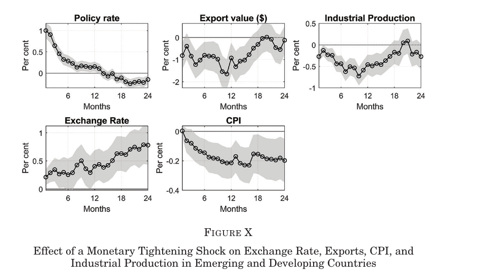
In the talk she read the same picture off the screen: “a tightening of monetary policy leads to an exchange appreciation and a fall in exports and industrial production” [00:47:40].

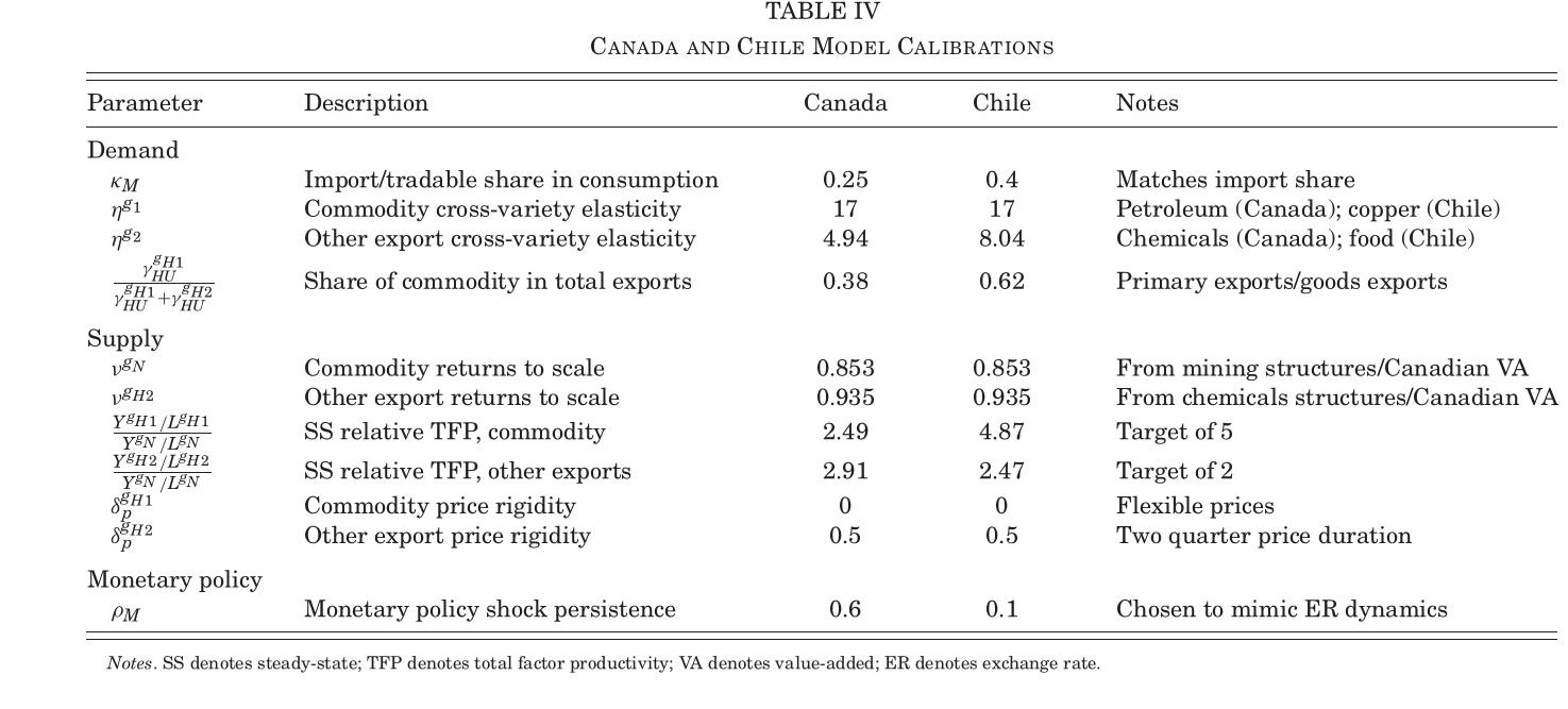
Second, Canada and Chile, chosen because both are commodity exporters invoicing mostly in dollars (70% and 94%) and both have usable shock series (Champagne and Sekkel’s narrative series for Canada, Brandão-Marques for Chile). A one-point Canadian tightening appreciates the loonie about 0.5%, and energy exports fall a peak of just over 1.5% at three months while chemicals fall over 1% at seven months — faster and larger for the more homogeneous, more flexibly priced good, which is what the model predicts and roughly reproduces once calibrated with separate elasticities (17 for petroleum against 4.94 for chemicals; the corresponding Chilean pair is 17 for copper against 8.04 for food). For Chile the appreciation peaks near 4% and mining exports drop about 10% on impact. One honest footnote: Canadian auto exports rise after an appreciation, which neither model explains.

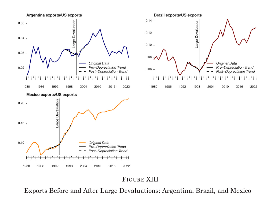
Third, three large devaluations — Mexico 1994, Brazil 1999, Argentina 2001, whose cumulative six-month depreciations against the dollar were 50%, 40% and 130% respectively (p. 659) — with exports normalized by US exports to strip out world trade. In each case exports had been flat or falling and then grew rapidly after the devaluation. These are endogenous events that happen in downturns when exports are already weak, so the authors argue the visible trend break is a lower bound.

Tenreyro added an unplanned fourth case from the floor: sterling after the Brexit referendum, when economists expected the tradable sector to suffer and instead, with productivity and trade barriers unchanged and only the exchange rate having moved, exporters had “a sweet spot.”

What the room pushed on

The questions were unusually good for a public lecture, and several of them were the same question. Jaume Ventura (if the captions have the name right) suggested looking at reallocation between tradables and non-tradables after a devaluation as a cleaner test of quantities; Tenreyro agreed and said they hadn’t done it. A second questioner pointed out that under strict DCP a monetary expansion should actually contract exports, because the domestic boom pulls inputs toward non-tradables while export demand is fixed — so the empirical prediction of that model is worse than “no effect,” and we never see it. Tenreyro thought that was right and noted the published DCP calibrations escape it only because some Calvo firms do get to reset. Someone asked whether one could invert the exercise and estimate how far reality sits from each paradigm by matching export impulse responses; she was open to it but pointed out that Canada and the emerging-market panel look about the same, which the model also delivers, so a third sticky-dollar category probably wouldn’t move much. A questioner asked whether this meant emerging markets shouldn’t manage exchange rates or use capital controls, and got the most carefully bounded answer of the afternoon: the claim is only that the exchange rate can stabilize, and “a country may still need to put capital controls for other reasons that are not in this paper” — but then present the mechanism and quantify it, because it isn’t coming from this one. And two questions she simply declined to answer — whether monopsony-laden commodity sectors let the benefit trickle down (a distributional question the model doesn’t touch) and whether dollar invoicing shares are trending (the time series is too patchy; their regressions are essentially cross-sectional).

The one odd thing

The genuinely surprising part is not that exports respond to exchange rates — that is the conventional wisdom of 1953 — but that a whole literature talked itself out of it using an observation that is equally consistent with either view, and then derived policy advice from the less plausible reading. Sixty years of micro evidence say competitive goods have flexible prices; forty-five years of invoicing theory say competitive goods are the ones priced in dollars; and the inference that went into the IMF’s report was that dollar-priced goods have sticky prices. The paper’s contribution is partly a model and partly a reminder that “the price didn’t move” has at least two explanations, and one of them is that nobody needed it to.

(Tenreyro’s own framing, in the talk’s last slide, was that most of the IMF’s clients are emerging and developing economies with high homogeneous-goods shares — which is to say the advice was being given most forcefully to exactly the countries for whom its assumptions are least true.)