Making Room on an Empty Planet: The Spatial Consequences of Depopulation

Tim de Silva and James Paron’s paper on depopulation starts from a prediction that nearly every quantitative spatial model makes and almost nobody says out loud. Take Japan. Remove nine-tenths of its people, evenly, and nobody moves. Tokyo keeps its 10% of the population, Hokkaido keeps its 4%, and every prefecture simply shrinks in proportion. Tokyo goes from 12 million people to 1 million. Nobody measured this. It comes from the functional forms: if housing supply and housing demand are both Cobb-Douglas, population shares are independent of the population level, and that is exactly the pair of assumptions the standard toolkit uses. The paper calls this property scale independence and treats it as something to be tested rather than assumed. Its answer is that shares do move, and they move toward the dense places. In their estimated model Tokyo ends up with 40% of a much smaller Japan, which is 4 million people rather than 1 million, and Hokkaido falls to 0.1% (pp. 3–4, 35).

A note on versions. The public paper is the authors’ working paper dated 21 August 2026 (the title page says the first draft dates from June). De Silva presented it at the nber virtual workshop on the macroeconomic effects of population aging on 18 September 2026, and Paron took most of the questions. Where the talk’s numbers differ from the paper’s, I use the paper’s and say so. De Silva was also clear about the scope: “this entire paper is going to be about the effects of changes in the population level. Nothing about the effects of population aging” (05:14:09).

What Japan did after 2010

Japan’s population peaked at 128 million in 2010, and by 2020 it was back around its 2000 level. Fertility averaged 1.35 over 2000–2023 (p. 8). De Silva said “around 1.2” in the talk (05:11:33), which is closer to recent years than to the paper’s average. The paper plots each prefecture’s change in log population share against its initial density (its population share over its share of inhabitable land), decade by decade. In the 1980s and 1990s, while the population was still growing, there is little relationship. In the 2000s and 2010s, as it levelled off and began to fall, the slope turns clearly positive. Tokyo’s share rose 1.6 percentage points between 2000 and 2019 and Hokkaido’s fell 0.3 points, mostly through internal migration of people in their twenties (pp. 9–10).

One country is an anecdote, so the paper also uses the Global Human Settlement Layer (Pesaresi et al. 2024), which counts population on a 1 km grid, to measure each country’s share of people living in high-density cells. Across countries over 2000–2020, faster population growth goes with a falling high-density share. The relationship survives country fixed effects in a five-year panel, which turns the Japan case study into a within-country regression (Table 1, p. 12; Table 2, p. 13). It also survives controls for the agricultural share and the old-age dependency ratio. The dependency ratio’s own coefficient is small and insignificant, which is how de Silva put it in the talk: the thing correlated with spatial allocation is “the level of the population rather than the dependency ratio” (05:19:20). These are reduced-form correlations, offered as motivation rather than identification.

The model: land as the weak link

The static model is a standard spatial equilibrium. Households draw Fréchet taste shocks (dispersion θ) and choose a location, where they consume goods and housing. Wages are A_i N_i^σ, so there is a local productivity fundamental and a little agglomeration. Housing is produced from a fixed stock of land and from structures built with local labour. Two forces concentrate people: some places are better, and scale helps. Two forces spread them out: taste shocks, and the fact that land is finite. As de Silva put it, “housing is a scarce resource that spreads people out” (05:13:47).

Now ask when national population N moves local shares N_i/N. Proposition 3 gives the general answer (eq. 17 in the paper, p. 21):

Here p_i h_i / w_i is the local housing expenditure share and ζ^S_i and ζ^D_i are the local price elasticities of per-capita housing supply and demand, with θ and σ as above. If nothing in the housing term varies across i, every region’s population moves one-for-one with the nation’s and shares are fixed. Cobb-Douglas supply and Cobb-Douglas demand make the share, both elasticities and therefore the whole term constant, and the paper shows this is the only case that gives scale independence for all primitives (Props. 1 and 3, pp. 17, 21). Once the term varies, regions where it is large track the national decline less closely. It is large where supply is inelastic and the housing share is high. So concentration rises as N falls if supply elasticities fall with density or expenditure shares rise with it (Prop. 4, p. 23).

The supply-side version is the cleaner of the two. Make housing a ces aggregate of structures and land with elasticity of substitution η. If η < 1 the two are complements, and the supply elasticity is ζ^S_i = ((1−ν)/ν)·η·(L_i/X_i)^{(1−η)/η}, which falls as structures pile up per unit of land (eq. 20, p. 21). In Tokyo there are plenty of structures and the constraint is land, so adding people mostly divides the same land more finely. In Hokkaido land is plentiful and extra people barely dent housing per head. Run it in reverse. A national decline raises land per head everywhere, but in Tokyo that land is the binding input, so housing per head rises a lot there and hardly at all in Hokkaido. People follow the housing. In de Silva’s words, these are places where “ideally you would build more housing, but you can’t because at some point you’re out of land” (05:25:56). Depopulation hands out land in equal parcels per head, and the parcels are worth most where land was the bottleneck.

The demand side has the same shape with the roles changed. Under homothetic pigl preferences housing demand is α w_i p_i^{−ζ_p}, so the demand elasticity is the constant ζ_p and the expenditure share is α p_i^{1−ζ_p} (eq. 22, p. 23). If ζ_p < 1, goods and housing are complements in consumption and the housing share rises with the house price, so it is highest in expensive, dense places. The expenditure share is a sufficient statistic for the marginal utility of housing (p. 20), so the same rise in housing per head is worth more in Tokyo. De Silva’s version: “if people are spending more on housing in dense cities by revealed preference they value housing more” (05:29:38). Tokyo has plenty of goods and not enough housing to enjoy them in. With ces supply and pigl demand together, eq. 17 becomes (eq. 23 in the paper, p. 23):

Here α p_i^{1−ζ_p} is the pigl housing share and ζ^S_i is the ces supply elasticity above. Density enters twice, through a lower ζ^S_i when η < 1 and a higher share when ζ_p < 1, and both push the same way.

The paper states the general ingredients well: you need complementarity plus differential returns to scale in N_i (p. 25). Structures scale with population while land does not. Goods scale with N_i^σ while housing scales less than one-for-one. The same logic applies to land-intensive agriculture and to public goods with shared capacity. A school or a fire station can serve many residents before it congests, so its cost per head falls with local population, and a shrinking sparse region finds it harder to keep one going (pp. 24–25). Anything that works like a fixed factor in dense places and like a scale economy in sparse ones produces the same result.

On the evidence for the two ingredients, de Silva was candid that there is no Japanese data: “We don’t have evidence on this from Japan. All we have is in the us” (05:29:49). Baum-Snow and Han’s (2024) us supply elasticities fall steeply with density, with a slope of −0.097 (0.008) against log density. Via eq. 26 that implies η ≈ 0.77, and the estimated model needs η = 0.65 to match it (pp. 26–27, 34). The expenditure-share evidence has a positive slope against log median income, +0.047 (0.008) (Fig. 4, p. 27), but de Silva called it “a bit more mixed” (05:30:28). ζ_p = 0.75 is calibrated from the midpoint of a range in the literature rather than estimated (p. 32). So the parameter that carries the paper, η, is identified off the American cross-section and then applied to Japanese prefectures, which is a normal thing to do and still worth keeping in mind.

Japan, emptied

The quantitative model makes the static one dynamic. It has 47 prefectures, forward-looking location choice with bilateral moving costs, a choice between working in goods and in construction, and durable structures that depreciate at 8% a year, all on top of ces housing and pigl preferences (Table 3, p. 29; η and δ from p. 34). Fundamentals are inverted to match 2000 population shares. The experiment holds population flat for twenty years and then lowers it at a constant rate to 10 million in 2195, under perfect foresight (p. 35). The talk said 2200 and added that the exact cutoff is “not super important” (05:33:37).

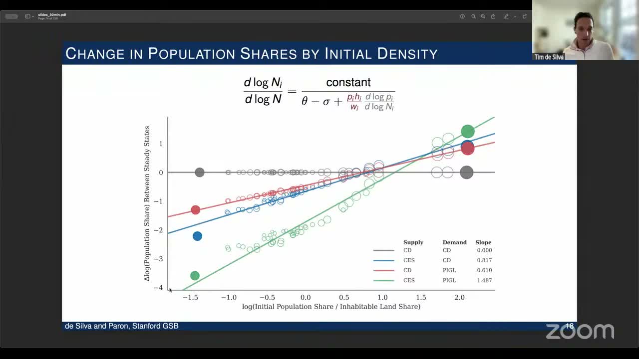
Every prefecture shrinks; the dense ones shrink far less. With both channels on, the slope of the change in log share on initial density is 1.487. ces supply alone gives 0.817, which is 55% of that, and pigl demand alone gives 0.610, or 41%. Cobb-Douglas on both sides gives exactly zero. The paper concludes that supply “contributes slightly more … and the interaction between the two is small” (p. 36). In the talk de Silva said about 65% and “40ish%” (05:35:00). The paper’s 55/41 is the arithmetic of the slopes on the slide.

Wages fall everywhere, because agglomeration is lost everywhere. They fall about 5% in Tokyo and about 25% in Hokkaido (p. 36). The wage slope divided by the share slope is roughly σ = 0.05 (p. 37), which says local wages are just local scale raised to the agglomeration elasticity. And yet:

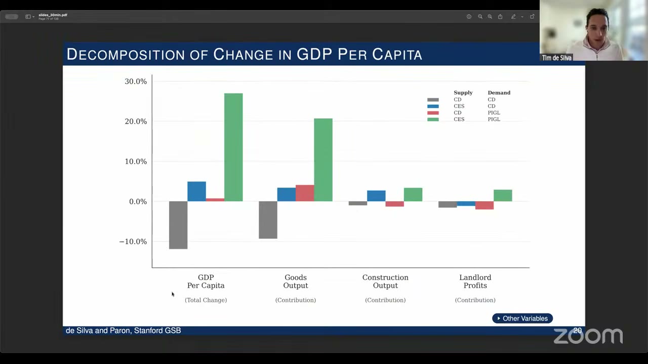
gdp per capita rises 26.9% in the baseline and falls 11.9% under scale independence (Fig. 7C, p. 38; the text rounds to 27%, and the talk said “25ish%” at 05:36:03). Wages fall in every prefecture but the average rises, and that is a composition effect. gdp per capita is the goods-employment share times scale N_Y^σ times an allocation term Σ A_i (N_iY/N_Y)^{1+σ} (p. 37). Scale falls in every model. The allocation term rises when people move into high-A_i Tokyo and Osaka, which the land constraint had been keeping them out of. The country gets richer by emptying its poorer places. One oddity: the share slopes nearly add up (0.817 + 0.610 against 1.487, which the paper notes), but the gdp gains do not: ces alone gives +4.9%, pigl alone +0.7%, and both together +26.9%. The paper does not comment on this, and I can’t reconstruct the reason from the main text. Prices show a different kind of cancellation. The supply channel makes house prices fall most in dense places and the demand channel makes them fall least there, and in the baseline the two nearly cancel, with a slope of 0.003 (Fig. 7D, pp. 38–39).

The transition is where the model meets the data, and it goes only partway. Moving is costly, so households move early to get ahead of future housing. Between 2000 and 2020, with national population still flat, Tokyo’s population in the model rises about 3% and Hokkaido’s falls about 3%, and Tokyo house prices rise (p. 39). The model’s density slope over this window is 0.017 against 0.079 in the data (p. 41). The paper calls that “approximately one-quarter”; the ratio is 22% (24% against the weighted data slope). De Silva said “around a fourth” and said other mechanisms, some of them in the next talk, must account for the rest (05:37:02). Birth rates and fundamentals are held fixed, although some of Tokyo’s real gain came from differential births. Full convergence takes more than two centuries after the decline ends, because structures depreciate slowly (p. 41). There is also a darker extension. With η < 1, housing per head is bounded above as population falls, so if fertility responds to housing it may never recover enough to stabilise the population. Under Cobb-Douglas it always does (p. 42).

The planner wants you in Tokyo

The planner is restricted to a wage-indexed transfer, τ_io = τ_w w_io + τ_0 (eq. 46, p. 43). In the static model the optimum is the Fajgelbaum–Gaubert (2020) trade-off between redistribution, which taxes Tokyo, and agglomeration, which subsidises it. At θ = 2.02 and σ = 0.05, redistribution wins and τ_w < 0 (Prop. 5, pp. 44–45). The dynamic model gets the opposite sign.

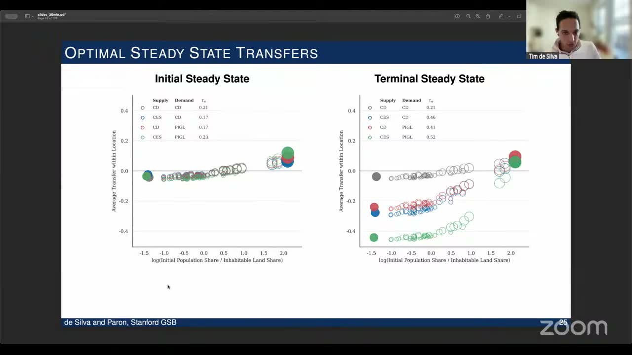
The optimal τ_w is 0.17–0.23 across the four models in the initial steady state (0.23 in the baseline). In the terminal steady state it is 0.52 in the baseline, 0.46 with ces only and 0.41 with pigl only, and it stays at 0.21 under Cobb-Douglas (Fig. 10, p. 44). The paper’s text says this means transfers of about 10% “of aggregate gdp” to Tokyo initially and about 5% at the end, with −45% in Hokkaido. That phrasing is loose about units. The figure plots the prefecture-average per-capita transfer, τ_w(w̄_i − w̄), in units where 2000 gdp per capita equals one (Fig. 10 notes, p. 44; normalisation p. 33). So the terminal “5%” means each Tokyo resident receives about 5% of 2000 gdp per head, and each remaining Hokkaido resident pays about 45% of it. It is not 5% of national gdp flowing to Tokyo. Tokyo’s per-capita transfer falls while τ_w doubles, presumably because once 40% of the country lives in Tokyo the national average wage is mostly Tokyo’s. Welfare gains go from 0.2–0.3% of lifetime consumption to 5.1% in the terminal baseline (p. 44).

The sign flip comes from moving costs, and Appendix F.6 checks this by removing the dynamic features one at a time (p. 45). Without moving costs, households arbitrage average utility across places. With them, average utility stays higher in Tokyo than in the sparse prefectures, so the planner gains by paying people to move there. Scale dependence widens that utility gap, so the payment grows. The paper notes that the policies actually in use point the other way. They include akiya banks, Italy’s 1-euro homes, and Scotland’s depopulation action plan (p. 46). The authors note that these are steady-state results and that abandoned homes and heritage values are outside the model (pp. 46–47). De Silva was careful about it too: “We don’t want to say that like the direction that … our model is spitting out is the right one” (05:39:58).

What the room pushed on

There was no discussant. The chair passed on a question from “Ron”, presumably Ronald Lee, about agriculture. If land frees up, does the marginal product of farm labour rise enough for rural areas to “fight back”? (05:41:12). Paron said the baseline has no sectoral differences in returns to scale. An extension with land-intensive, low-agglomeration agriculture amplifies concentration rather than resisting it (05:41:55).

The sharpest exchange came from a participant the chair called “Yui” (the captions may have garbled the name). The questioner separated two things inside the ces. One is the cross-section, where supply elasticities differ by density. The other is the time series: as land becomes abundant, its value share in housing falls, so the economy depends less on the very input that disperses people. He asked which matters more (05:42:43). The reply (captions do not make clear which author gave it) was that these are the same mechanism described two ways (05:44:21). The questioner said they are generated by the same assumption but are different channels, and left it as a comment (05:45:02). It was not resolved. I think the questioner has a point: one parameter producing both a cross-sectional and a secular prediction is economical, but it also means one estimate, η, disciplined by us cross-sectional data, carries both.

The same questioner also asked why moving costs should change optimal policy, since they are a real cost the planner bears too (05:45:42). Paron answered that “the reason” referred to the difference between the static and dynamic results. Moving costs leave a utility gap that households cannot arbitrage, and the planner pays them to bear the cost of closing it (05:46:22). The questioner said they would check the paper. It is a fair question. A household already weighs its own moving cost against its own gain, so for the planner to want more moves than households choose there has to be a wedge somewhere, and the main text gives the first-order condition without saying what the wedge is.

A participant the chair called “Will”, presumably Will Dow, asked about Tokyo’s large, slowly depreciating stock of past investment (05:47:46). Paron pointed to the spending-commitments extension. Public goods with adjustment costs are hardest to fund where the tax base is shrinking fastest, which is the rural areas, and this amplifies the anticipation-window responses by about 15% (p. 42). De Silva added that slow depreciation of structures is the reason the model is dynamic and that it “substantially quantitatively slows down the transition” (05:50:10).

The upshot

The paper’s claim is not that Tokyo is special. It is that the standard model, by assuming Cobb-Douglas, rules out any spatial effect of population size, and that the mechanism the assumption removes is large: it moves Tokyo from a tenth of Japan to two-fifths. Governments are currently paying people to stay in rural areas, and the model’s planner would pay them to leave. The paper is careful not to recommend that. Its point is narrower: once you stop assuming the answer, rural-retention policy needs a justification that the standard model never had to supply.

References