Do Online Job Postings Capture Job Vacancies?

You have the near-universe of American job ads. Forty thousand job sites scraped, deduplicated, parsed into skills and education requirements and posted salaries, available in something close to real time, and fine enough to cut a commuting zone by a four-digit industry — the granularity the official vacancy survey cannot dream of, since jolts is about 16,000 establishments each sitting in the panel for 24 months. A decade of labour economics has been built on this, and for good reason. There is exactly one thing you cannot do with it, which is ask whether the establishments that post ads resemble the establishments that have openings. The ad gives you an employer name and a location and then stops. No size, no age, no wage bill. So every validation anyone has run has compared aggregates — Burning Glass by industry against jolts by industry, by occupation, by state — and every one of them has been silent on the only question that matters for a statistic computed across employers.

Michael Dalton of bls, Lisa Kahn of Rochester and Andreas Mueller of Zurich went and got the employer characteristics. They match Burning Glass ads to the Quarterly Census of Employment and Wages — the business registry behind every bls establishment survey, covering more than 95% of jobs — on cleaned employer name crossed with location, and because qcew is the jolts sampling frame, jolts arrives attached. Kahn presented it on the first afternoon; it is a conference draft dated 22 August 2026 and an nber working paper, and it is preliminary in the ordinary way. Matt Sigelman is thanked in the acknowledgements for providing the data, which will become funny in about nine hundred words.

First the concept mismatch, because everything downstream is a consequence of it. Burning Glass is a flow of new ads. jolts is a stock — unfilled positions on the last business day of the month, actively recruited, startable — plus a separate flow of hires. These are not the same object and no amount of scraping makes them one. The paper converts the stock to a flow with a law of motion: openings this month are hires this month plus the change in unfilled vacancies, which they call $N$ and which is deliberately an upper bound, because a hire that never had a posted vacancy behind it gets counted in. The alternative, using unfilled vacancies alone, would be a lower bound. Postings get averaged over a three-month window centred on the jolts month so that time aggregation does not do the work. Then there is the merge itself: 69% of postings carry an employer name plus a geographic identifier at least as fine as state (the missing 30% are mostly recruiters keeping a client confidential), and 91.6% of those find at least one qcew establishment. Kahn rounded both in the talk — “about 70 percent”, “more than 90 percent” — and passed over the machinery in one sentence: “Mike Dalton likes to say that this is two years of his life that is now relegated to a footnote.”

The mechanism, as a probability tree.

Here is why the paper is a model paper and not a regression. If you take the matched micro-data and regress jolts openings on Burning Glass postings at the establishment-month, you get almost nothing, because establishments with openings frequently do not post and a great many postings come from establishments with no openings. Both errors are enormous and neither is a rounding term. So the authors write down the smallest possible data-generating process instead. An establishment of type $j$ — a bundle of qcew observables: sector, wage quintile, urbanicity, age, growth, a size spline, local characteristics — has openings with probability $p^N$, and conditional on having them posts online with probability $p^B$, putting up $B^+$ ads. With no openings it may still post, with probability $p^{B0}$, putting up $B^0$ ads. Four leaves, and each one is a named failure mode: matched, where both datasets see the same employer; invisible, recruiting with no ad; spurious, an ad with no opening; and neither, which is in no dataset and which exists so the probabilities sum to one.

Take expectations and the whole thing collapses to one multiplicative wedge:

where $1/p^B$ is the extensive margin (scale up the employers who never advertised), $n = N^+/B^+$ is the intensive margin (how many jobs one ad is worth), and $s^B$ is the nuisance share — the fraction of expected postings that come from establishment-months which actually have a jolts opening, a deflator into which merge error, time aggregation and definitional mismatch have all been swept together. Six moments generate all three, estimated by probit and exponential-mean regression on type. Crucially, every covariate lives in the qcew, so a model fitted inside the small jolts intersection can be pushed out to the entire Burning Glass–qcew match and used to predict openings as $\hat{a} \cdot B$. That is the trick that buys commuting-zone-by-four-digit-industry granularity out of a 16,000-establishment survey.

What the wedge looks like. About 28 in 2007 — one average establishment’s posting had to be multiplied by 28 to reach an average jolts opening — down to 10 by 2011 and around 4 for the rest of the sample, with Kahn dating the end of the steep decline to about 2013. Averaged over the stable 2011–19 window, which is when most of the applied literature was written, it is 6.2. The dashed composition-adjusted series declines just as steeply, so this is not a story about which kinds of employers happen to be hiring; employers of a fixed type genuinely got better at advertising online.

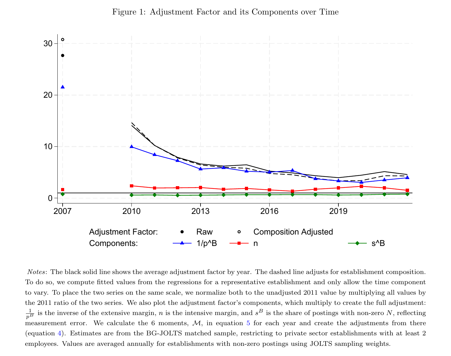
The decomposition is where it stops being comfortable. The extensive margin does essentially all the converging, falling about sevenfold and ending near 3 — meaning that even at the end of the sample, roughly one recruiting establishment in three posts online. The intensive margin is flat at about 2, so one ad is about two jobs. And the nuisance share is flat at about 0.6, which is to say that about 40% of online job postings come from establishment-months with no corresponding jolts opening at all. Both mismatches live in small firms and both terms go to 1 for large ones, which is the entire paper in one clause. Cross-validation inside jolts is reassuring about what it is designed to be reassuring about: raw postings track predicted openings with a slope of 0.149 in and out of sample, adjusted postings with 0.996 and 1.002. That validates predictable group means, not establishment-specific fit, and the paper says so.

The gradients are steep and they are all the same gradient wearing different clothes. Across wage bill per worker, the bottom quintile needs a factor of 17 and the top 2.8. Across urbanicity, a large central metro needs 4.5 and a noncore area about 16, and local skill and economic-health controls do not touch it. Across size, the largest establishments need about 3.6 and mid-sized ones roughly double that. The gradient does not continue into the very smallest bins, which also land near 6, and Kahn was careful about why: for those establishments a very low posting probability is offset by a very low nuisance share, the two errors cancelling for no good reason. “The smallest firms are sort of where we’re having this issue with our nuisance parameter,” she said, and flagged in advance that “any conclusions I’m going to tell you later are not dependent on these smallest firm bins.”

The good news, which is real. Kahn’s phrase for the result is a white-pages/yellow-pages story. Large establishments post well and account for most openings; small establishments post badly and account for most establishments. So anything you compute over the distribution of openings is in decent shape. Skill demand moves, but modestly: the professional-occupation share falls from 0.45 to 0.38 under reweighting, the education requirement from 0.56 to 0.50, computer skills from 0.37 to 0.30, cognitive from 0.31 to 0.26, blue-collar rises from 0.12 to 0.16, and the conditional average posted salary drops from 49,405 to 46,234. Six or seven points, in the direction you would guess. And the Hershbein–Kahn upskilling result — which is Kahn’s own, and which leans its entire pre-period on 2007, the single worst-represented year in the data — survives. Post-recession increases in demand for automation-related skills and their persistence both hold after reweighting and, the paper says, if anything strengthen. An author reweighting her own famous result and finding it intact is the sort of thing that should be reported more often, including in the cases where it doesn’t happen.

The casualty is labour-market concentration. Researchers took the breadth of online postings and computed Herfindahls of hiring employers at fine geographies, and that literature has moved academic and policy debate toward employer market power. A Herfindahl is a sum of squared shares, which makes it a statistic about the distribution of employers, not of openings — precisely the object the white-pages half of the story says is wrong. Squaring makes the missing tail decisive. Markets here are four-digit naics by commuting zone by month, pooled 2011–19, and the adjusted index uses a second-order analogue of the wedge on the numerator with the first-order one predicting market size in the denominator.

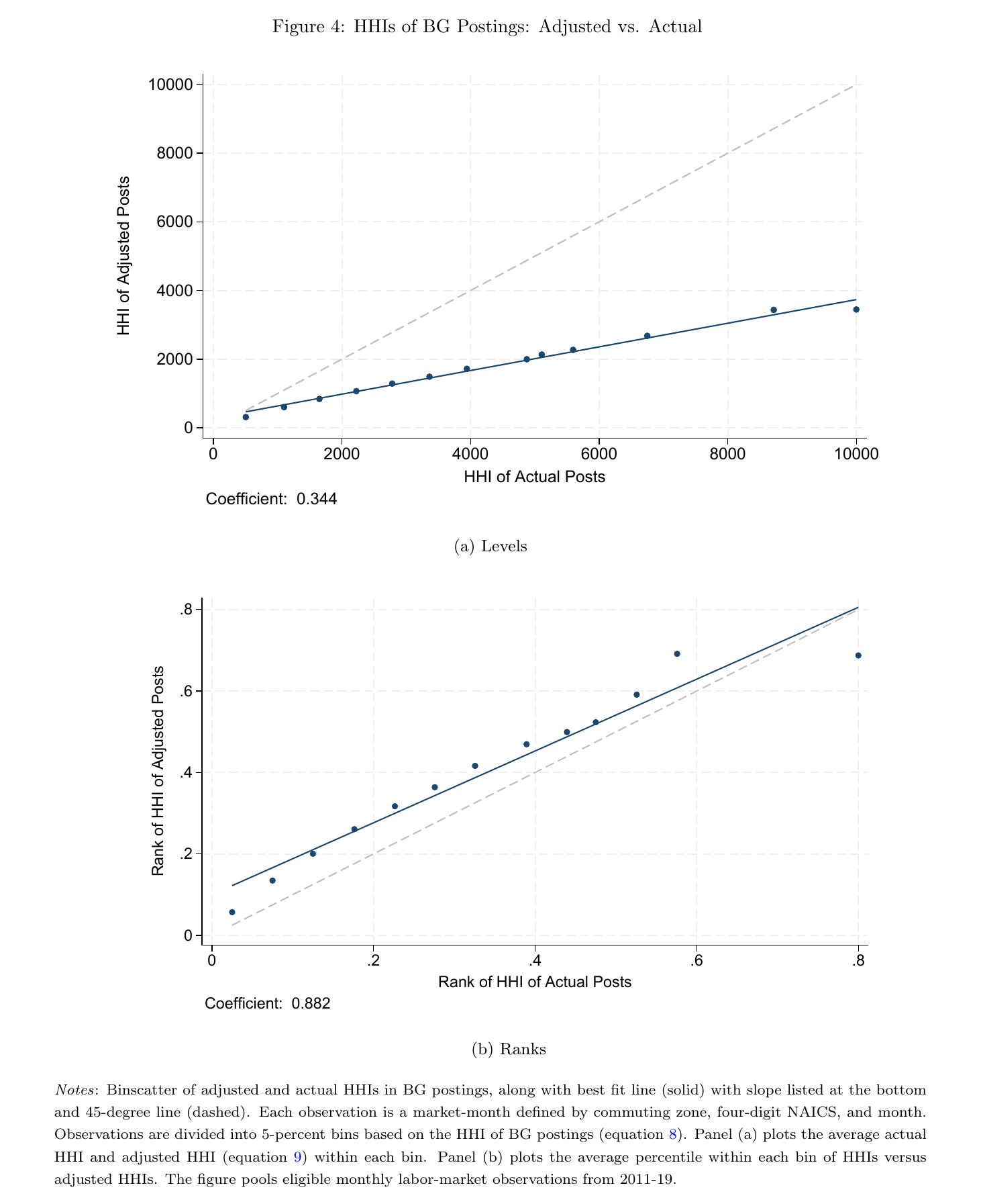
“The slope of this line is about point three and far below the 45 degree line,” Kahn said. “The level of labor market concentration needs to be scaled down to about a third of what you would measure in Burning Glass.” The robustness checks all land in the same place: 0.350 excluding establishments under ten employees, 0.379 weighting markets by employment, and between 0.269 and 0.344 across quartiles of predicted market size. There is also a genuinely independent check — simulate qcew-sized markets out of jolts establishments, where the true openings are observable, and the Herfindahl of actual openings on the Herfindahl of postings has a slope of 0.389, which the adjusted index reproduces at 0.392.

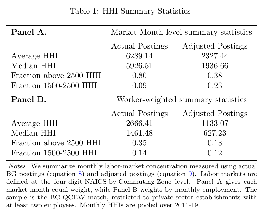
Keep the two panels apart, because the headline number everyone remembers lives in the first one. Counting market-months equally, 80% of American local labour markets sit above the 2010 doj/ftc threshold at which a market is called highly concentrated. Adjust for who actually advertises and that becomes 38%, with the moderately concentrated band swelling from 0.09 to 0.23 as markets fall into it from above. Average concentration drops 63%. Weighting markets by employment instead — the worker’s-eye view — the raw share above the threshold is already only 35%, and adjustment takes it to 13%, a 57% fall in the average. Most workers, on these numbers, do not live in highly concentrated labour markets. The paper is also scrupulous that its unadjusted 80% is not the 60% of Azar et al., who restrict on market size and define markets by occupation; this universe includes single-poster markets sitting at the maximal 10,000, which pushes the raw share up. That footnote matters, and it does not rescue the level.

What it does rescue is the literature’s regressions. Rank correlation is 0.882, and 1.011 when employment-weighted. “If you want to put a Herfindahl on the right hand side of your regression you’re going to capture meaningful variation,” Kahn said. “One should just not take seriously the level of concentration, which people have tended to do.” Which is an unusually clean division of the spoils: the identification survives and the sentence in the policy memo does not.

The discussant. Gad Levanon of the Burning Glass Institute had both Session 3 papers, and opened with a disclosure that should be preserved for posterity. His organisation and the organisation whose data this paper uses are, he explained, “completely two different organizations”; they share a name only because Matt Sigelman ran the one and is president of the other; “if anything there is a mutual feeling of hostility and animosity between the organization — they indeed sued us to want us to change our name.” Then he called it “probably the best paper we have on the biases of online job openings” and made four points.

The first is the one the authors should worry about. A user can already adjust raw postings using published jolts breakdowns by industry and region, for free, without a restricted-access micro-merge. How much better is this? Levanon expects it is better — “because you have information on variation within industry and that you can’t just do with jolts” — but wants the comparison shown. There is no author response on record; the shared Q&A went to the other paper.

The second cuts against the paper’s own headline. Levanon, apropos of his hair, offered quality scores: qcew at 97, ces at 90, “levels of posting are at 70 and time series of posting are like 13, 14.” Most users of postings look at changes over time, not levels, and the method here fixes cross-sectional representativeness. To fix the time series “there’s a lot of unglamorous work in dealing with things like job posting coming and going, scraping from other job boards, all kinds of non-economic reasons.” Note what this implies about Figure 1: the 28-to-4 convergence is itself a posting time series, which is the series Levanon trusts least. The paper’s defence is the composition-adjusted line, but that controls for who is posting, not for how the scrape changed.

Third, publish the weights — “or better if bls publishes those weights and takes over this” — escalating to his big-and-bold idea that bls should simply run a job-postings programme of its own. Kahn had pre-empted the first half in the talk: they fit a second version using only characteristics available in Burning Glass itself, “because researchers won’t have access to this merge in practice,” and are “working on being able to release those weights.” Fourth, the method is bigger than the paper: any private dataset with an identified employer can be audited this way, adp included, and he offered up his own institute’s data to be audited.

From the floor, one question on this paper. An unnamed questioner went straight at the nuisance parameter: some firms go fishing — permanently posted, rarely hiring — so could you identify the always-posting, never-hiring establishments and remove them? Kahn’s answer was careful and conceded the right amount. Those establishment-months have neither hires nor unfilled vacancies under a definition that requires active recruiting, so she does not read them as phantom vacancies. The live version of the worry is recycling: Lightcast treats an ad still up after 60 days as a new posting, and “it’s like fast food, there’s always having those things up.” They checked, and the industry pattern does not cooperate — food and accommodation services does not have a particularly high nuisance factor. Then the concession: she has not yet crossed recycling rates with establishment size, which is exactly where the mismatch concentrates.

So the standing of the scraped-ads literature after this paper is roughly as follows. The ads are a fine sample of jobs and a bad sample of employers, the gap has been closing for fifteen years, and the one result that depended on counting employers rather than jobs was the one that got quoted in merger guidelines. Levanon is right that the remaining work is unglamorous, and he is right about who should be doing it, which is a conclusion that requires a functioning statistical agency with a budget — a thing this conference had spent the previous two sessions establishing the United States no longer reliably has.