Long-Run Productivity Risk: A New Hope for Production-Based Asset Pricing?

Mariano Massimiliano Croce, Journal of Monetary Economics 66 (2014), 13–31. Published version, with online appendix; no recorded talk.

Mariano Massimiliano Croce’s paper asks where the long-run risk in Bansal and Yaron (2004) comes from, and gives the most direct answer available: from productivity. Bansal and Yaron work in an endowment economy. Consumption and dividends simply arrive, with a small, very persistent drift in expected growth, and an Epstein–Zin (1989) investor who cares about the timing of resolution of uncertainty is terrified of that drift. That gets you an equity premium and a low risk-free rate, and it leaves an obvious question hanging: why should consumption have that drift? In a production economy consumption is a choice. A planner who sees bad long-run news coming can reallocate, save, work, and smooth, and the familiar experience in this literature is that a planner who can smooth tends to smooth the equity premium right out of existence.

Croce’s move is to push the drift one layer down. Put the small persistent component in total factor productivity, let consumption, investment, hours and Tobin’s q be chosen, and see what survives. The answer is that the premium survives, but only if two things hold at once: the elasticity of intertemporal substitution has to be high enough that good long-run news makes you invest rather than consume, and installing capital has to be convexly costly so that the investment boom shows up as a capital gain. Take away either and the premium collapses or changes sign. In the arc of this reading collection the paper is the bridge: Bansal and Yaron posit the drift in consumption, Croce relocates it to tfp and treats it as exogenous, and Kung and Schmid (2015) make it endogenous by having R&D produce it. Croce says as much in his conclusion, noting “good reasons to believe that these long-run components are endogenous” and pointing to the working-paper version of Kung and Schmid. He does not claim to have explained the drift. He claims it is in the data and that a production economy can price it.

Looking for the drift in productivity

The productivity process is Bansal–Yaron’s consumption process with the labels changed:

This is eq. 1 in the paper: $\Delta a$ is log productivity growth, $\mu$ its mean, $x_t$ the persistent conditional mean with persistence $\rho$, $\sigma\epsilon_a$ the i.i.d. short-run shock and $\epsilon_x$ the long-run news, with correlation $\rho_{xa}$ between the two.

The trouble with $x_t$ is that it is small and latent, which is the whole point of it and also the whole problem. Croce estimates it four ways on annual data through 2008 (stopping before the Great Recession), using three productivity series: Solow residuals from 1930, the bls multifactor measure, and the Basu, Fernald, and Kimball (2006) utilisation-adjusted series, both from 1950.

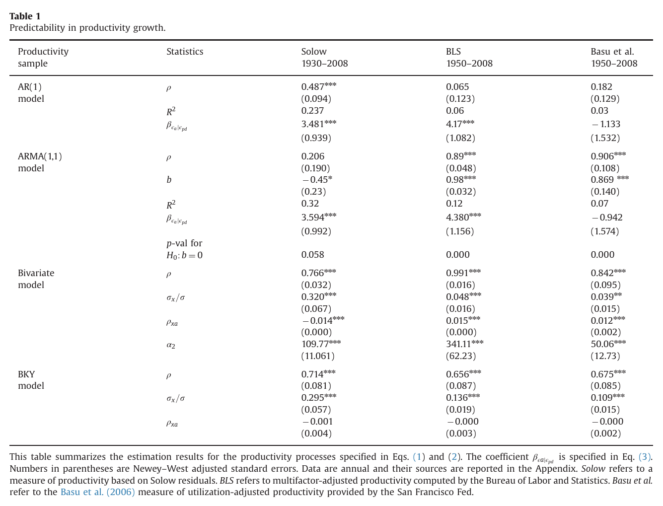
Table 1 is worth reading from top to bottom, because the answer depends heavily on how you look. A plain ar(1) on productivity growth finds persistence of 0.487 in the Solow series and essentially nothing in the other two (0.065 and 0.182, insignificant, with $R^2$ of 0.06 and 0.03). An arma(1,1) finds $\rho$ near 0.9 in the bls and Basu series, but with moving-average coefficients of 0.98 and 0.869, which is the near-cancelling case that is very hard to tell apart from white noise. Neither univariate filter can separate the two shocks; both force $\rho_{xa}=1$ by construction. The persistence becomes robust when asset prices are allowed to help. The bivariate filter estimates eq. 1 jointly with an equation for the log price-dividend ratio and gets $\rho$ of 0.766, 0.991 and 0.842. The Bansal, Kiku, and Yaron (2010) approach regresses next year’s productivity growth on the risk-free rate and the price-dividend ratio, calls the fitted value $x_t$, and gets $\rho$ around 0.66 to 0.71 with $\sigma_x/\sigma$ between 0.109 and 0.295. So the long-run component is, in a fairly literal sense, the part of productivity growth that the stock and bond markets forecast. Hold that thought for the weak points.

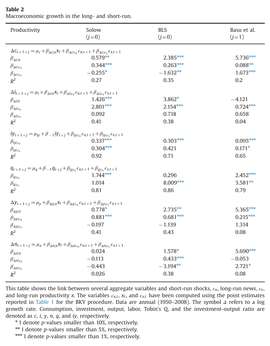
Table 2 then regresses macro quantities on the extracted pieces. The long-run component loads positively and significantly on consumption growth (0.579, 2.385, 5.736 across the three series) and on output growth, which is what you want if $x$ is a real drift rather than a statistical artefact. It is less tidy elsewhere: the loading of investment growth on $x$ is −4.121 and insignificant in the Basu column, and hours load on it with 0.024 in the Solow column. The interesting row is the immediate response of consumption to long-run news, $\beta_{\Delta c|\epsilon_x}$: −0.255 for Solow, −1.632 for bls, and +1.673 for Basu. Two of three measures say consumption falls when good long-run news arrives, and the utilisation-adjusted one says it rises. Croce notes this dependence himself. It matters, because the model is going to take a side.

The mechanism: an investment boom against an upward-sloping supply of capital

The model is a one-sector real business cycle economy solved as a planner’s problem. Output is $Y=K^\alpha(An)^{1-\alpha}$, with $\Delta a$ following eq. 1 at a monthly frequency. The household has Epstein–Zin–Weil preferences over a Cobb–Douglas bundle of consumption and leisure, with risk aversion of 10 and an ies of 2. The one non-standard piece is capital accumulation, which carries a Jermann (1998) adjustment cost:

These are eqs. 4–5 in the paper: $G_t$ is the fraction of capital lost in installation, convex in the investment rate $I_t/K_t$, $\xi$ is the elasticity of the investment rate with respect to the price of capital (set to 7), and $\alpha_0,\alpha_1$ make the cost and its slope zero at the steady state.

The cost matters because of what it does to the price of installed capital:

This is eq. 7 in the paper: $Q_t$ is Tobin’s q, the rate at which consumption goods turn into installed capital, and $G'_t$ the slope of the installation cost in the investment rate, so $Q$ rises whenever investment rises above its steady-state rate.

So the supply of new capital slopes up. When investment demand jumps, $Q$ jumps, and the holder of installed capital gets a capital gain. Without the cost, $Q\equiv1$ and the return on capital is just the marginal product plus undepreciated capital, which barely moves on news about the far future.

Now feed it long-run news. You are the planner, and you learn that productivity growth will be slightly higher for the next several decades. Two things pull in opposite directions. Capital is going to be more productive, so you would like to consume less now and invest more (substitution). You are also much richer, so you would like to consume more now (income). Which wins depends on the ies. With $\Psi=2$, substitution wins: consumption growth dips on impact, investment and hours rise, and, because investment is costly to install, $Q$ rises. Meanwhile the continuation value jumps, because a persistent improvement in growth is a large improvement in lifetime utility, and with $\gamma>1/\Psi$ the stochastic discount factor falls sharply. The return on capital is high exactly when marginal utility is low. That is a bad hedge, and bad hedges earn premia. In Croce’s words, the Euler equation implies $E_t[r_{t+1}-r_{f,t}]\approx-\text{cov}_t(m_{t+1},r_{t+1})$, and the covariance comes mostly from long-run news.

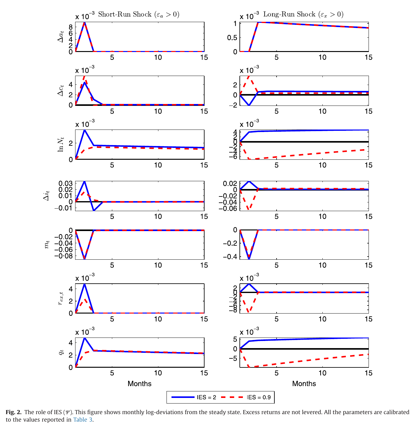
Fig. 2 shows it. On the short-run side (left column) everything moves together, as in any rbc model, and the ies barely matters. On the long-run side (right column) the solid line has consumption growth briefly negative, investment and $q$ up, the log sdf down by about 0.4, and the excess return up. The dashed line, with $\Psi=0.9$, is the mirror image on the quantities that matter for pricing: investment growth falls to about −0.06, $q$ falls, and the excess return goes negative.

A useful side effect falls out of the same mechanism. Short-run shocks move consumption and investment together. With a high ies, long-run news moves them apart. Mix the two and you get a moderate correlation, which is what the data show at annual frequency and what standard rbc models notoriously do not.

The evidence

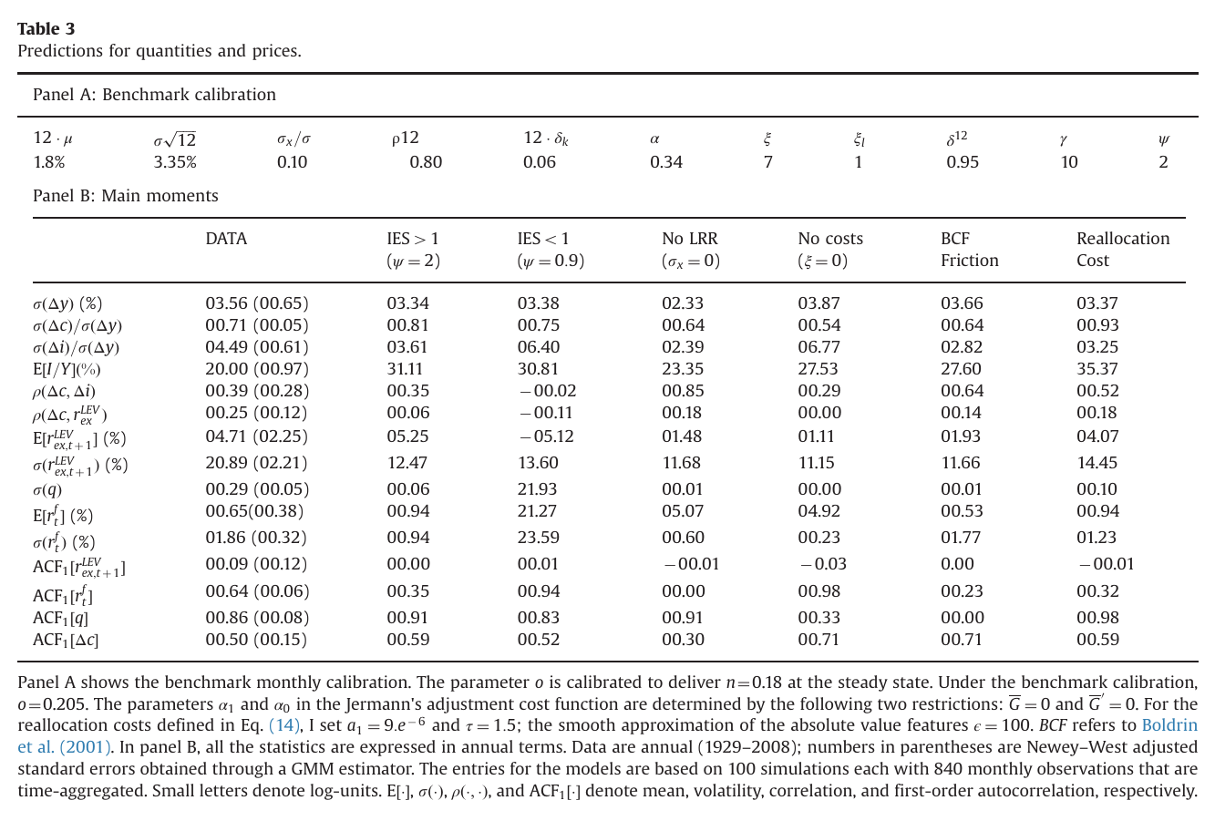
Table 3 is the paper. The benchmark is calibrated monthly with $\rho^{12}=0.80$, $\sigma_x/\sigma=0.10$, $\xi=7$, $\gamma=10$, $\Psi=2$ and time-aggregated to annual moments over 100 simulations of 840 months. Its levered equity premium is 5.25% against 4.71% in the 1929–2008 data, with a risk-free rate of 0.94% against 0.65%. The correlation of consumption and investment growth is 0.35 against 0.39. The correlation of consumption growth with levered excess returns is 0.06, against 0.25 in the table’s data column. That last number is the selling point: the premium does not come from a large contemporaneous consumption beta, which is how production economies with habits have usually gotten one, but from exposure to news about the long run. The risk-free rate is also smooth (volatility 0.94% against 1.86%) and persistent, if less so than in the data (autocorrelation 0.35 against 0.64), which is a real improvement on habit-based production models whose risk-free rates swing wildly.

The ablation columns tell you which parts are load-bearing. Turn off long-run risk ($\sigma_x=0$) and the premium falls to 1.48%, the risk-free rate rises to 5.07%, and the consumption-investment correlation goes to 0.85. Turn off the adjustment cost and the premium is 1.11%, because $Q$ cannot move. Lower the ies to 0.9 and you get a premium of −5.12%, a risk-free rate of 21.27% and a $q$ volatility of 21.93, which is less a calibration than a cry for help.

The sensitivity analysis in Table 4 adds two more numbers worth knowing. If you replace the latent long-run component with an ar(1) for productivity growth with $\rho=0.5$, the premium is 2.26%. An arma(1,1) gives 8.34%, but the author attributes this to the forced $\rho_{xa}=1$ rather than to anything you should believe. Moving to a quarterly decision interval at the same annual persistence costs 290 basis points of premium, which is recovered only by raising quarterly persistence to $\rho^4=0.90$. Adding stochastic volatility uncorrelated with news lowers the premium by 35 basis points, unlike in the endowment economy, because investment rises when uncertainty rises and equity hedges volatility shocks.

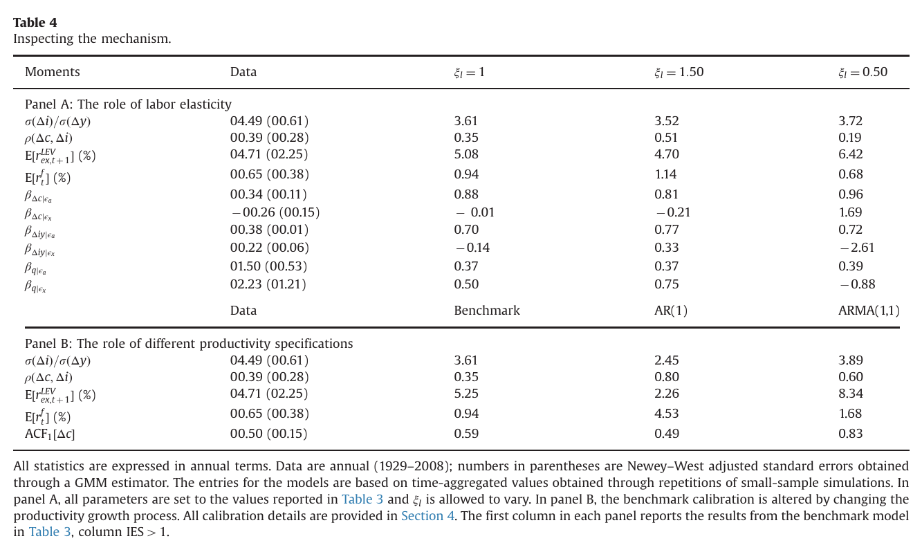
Panel A of Table 4 also confesses something small. Croce re-runs the Table 2 regressions inside the model, on annual Solow residuals computed from simulated data and re-filtered with the bky projection, and the estimated exposure of the investment-output ratio to long-run news comes out negative ($-0.14$ against 0.22 in the data), even though the structural response of $I/Y$ to long-run news is positive (Fig. 3b). A consumption-leisure elasticity above one, “although not necessarily as high as 1.50”, fixes the estimated sign (0.33 at 1.5) at the cost of a slightly lower premium (4.70%).

The one surprising thing

The ies sets the sign of the equity premium, not just its size. In the endowment economy a low ies is a nuisance: it weakens the long-run risk channel and does bad things to the risk-free rate. Here it reverses the channel. With $\Psi=0.9$, everything else unchanged, good long-run news makes the household consume its new wealth by cutting investment, $Q$ falls, and the return on capital falls at the same moment the discount factor falls. Croce’s phrase is that the market then “functions as an insurance device with respect to long-run news”, and insurance pays a negative premium. The paper computes only $\Psi=2$ and $\Psi=0.9$ and says the substitution effect wins when the ies is “sufficiently high”. So “the ies must exceed one” is a natural reading of the two columns, not a threshold the paper computes. But the direction is clear, and it gives the production version of long-run risk a sharper empirical commitment than the endowment version: it needs investment, and with it $Q$, to rise on good long-run news. Table 2 says investment-output and $q$ do load positively on long-run news, mostly significantly, so the commitment is at least not contradicted.

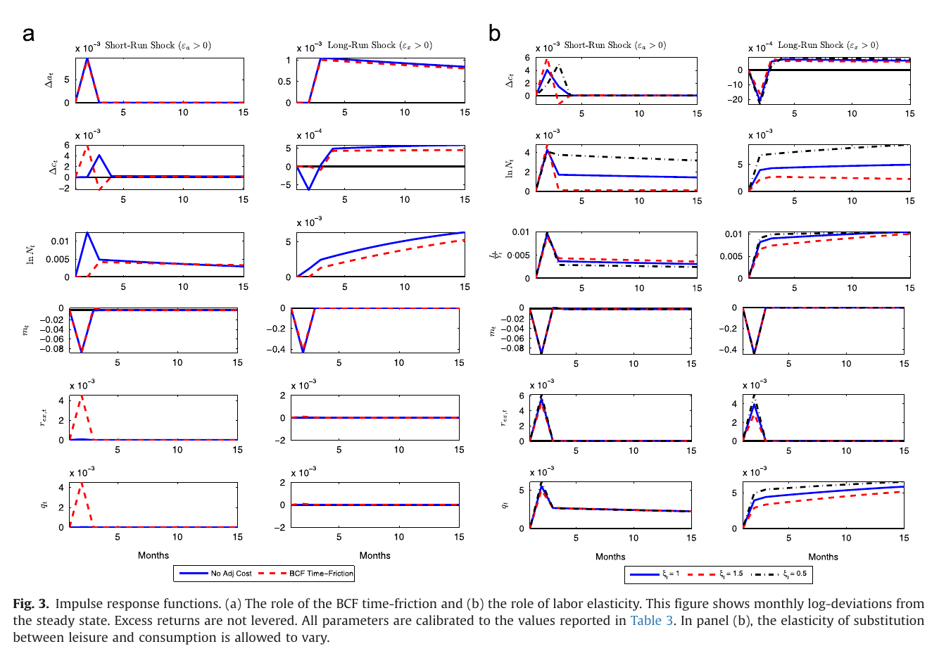
The runner-up is the friction horse race. The classic way to make $Q$ volatile in a production economy is Boldrin, Christiano, and Fisher’s (2001) time friction: the investment share of output and hours are chosen a period in advance. That works well against short-run shocks, as Fig. 3(a) shows: $q$ spikes on impact. Against long-run news it does essentially nothing, and the paper puts the response of $q$ “in the order of” $5\times10^{-5}$. The reason is obvious once said. Long-run news is tiny on impact and lasts for decades, so being forced to wait one month before adjusting investment costs you almost nothing. The premium is 1.93%. Keep the two-sector idea but make reallocation contemporaneous and convexly costly, $G_t=[a_1|S_t-\bar S|]^\tau$ with $S_t=I_t/Y_t$, and the price of capital becomes $Q_t=1/(1-G'_tK_t/Y_t)$ (eqs. 14–15 in the paper). That is increasing in the investment-output ratio, the correlation of Tobin’s q with $I/Y$ is positive in the data (0.605 in the paper’s Fig. 5a), and the premium comes back to 4.07%, with reallocation costs averaging under half a percent of output. What matters is a convex, contemporaneous price for moving resources into investment, not a delay.

Weak points, my own reading (no discussant exists)

The first is a circularity worth being explicit about. The univariate evidence for a persistent component in productivity growth is weak: the ar(1) persistence is insignificant in two of three series, and the arma estimates sit in the near-cancelling region. The robust persistence comes from the bivariate and bky filters, which identify $x$ from the price-dividend ratio and the risk-free rate. The model is then judged on how well it prices equity. That does not make the exercise wrong (it is a fair use of forward-looking prices to extract expectations), but the empirical support for long-run productivity risk is not independent of asset prices, and the price-dividend loadings in Table 1 are partly built in by construction. The estimated $\sigma_x/\sigma$ also ranges from 0.039 to 0.320 across methods and series, and the calibration picks 0.10, a sensible point in a wide interval. The bivariate $\rho_{xa}$ estimates are tiny but starred with standard errors printed as 0.000, and the paper says nothing about them.

The second is volatility. Equity return volatility is 12.47% in the model against 20.89% in the data, and $q$ volatility is 0.06 against 0.29. Croce is upfront about the trade-off: a stiffer friction makes prices volatile and quantities smooth, and $\xi=7$ is chosen mild to fit investment volatility. The less advertised consequence is in the Sharpe ratio. A 5.25% premium on 12.47% volatility is about 0.42, against about 0.23 in the data, and that is after adding an unpriced dividend shock with 6.5% annual volatility and leverage of 2, which the paper adds because “without this shock, the equity Sharpe ratio becomes excessively large”. So the priced part of returns is too smooth and earns too much per unit of risk.

Third, the model takes a side on the consumption response to news that the data do not settle. With the ies high enough, consumption falls on good long-run news; Table 2 agrees for Solow and bls and disagrees for the utilisation-adjusted series. A Beaudry–Portier (2006) news boom in which consumption and investment rise together is ruled out, and the author leaves the frictions that might allow it to future work.

Fourth, some small inconsistencies. The text puts the data correlation of consumption growth and excess returns at “about 21%” while Table 3 prints 0.25. Table 3 heads the frictionless column “No costs ($\xi=0$)”, while the text removes the costs with $\xi\to+\infty$, which is the right limit given that $\xi$ is the elasticity of investment to $Q$; the header looks like a typo. Table 4 says its data column comes from Table 2, but several numbers differ (the $q$ loading on long-run news is 2.23 in one and 1.014 in the other), and its Panel A benchmark premium is 5.08% where Table 3 and Panel B print 5.25%. The text calibrates $\sigma$ at 1% a month, while Table 3 prints $\sigma\sqrt{12}=3.35\%$ rather than 3.46%. And the paper says the model is solved by perturbation in dynare++ without saying to what order, which matters, since a first-order solution has no risk premium at all.

Finally, the long-run component is a free exogenous process with its own two parameters, chosen to match. That is the point the conclusion concedes and the point the next paper in this collection takes up. Croce shows that if productivity has a small persistent drift, a production economy with the right ies and the right friction will price it at roughly the size of the equity premium. Why productivity should have such a drift is somebody else’s paper.

That is a fair division of labour, and it is roughly how the literature went. Bansal and Yaron put a slow, scary drift in consumption and asked you to accept it. Croce showed that you can move it into technology, let a planner who would very much like to smooth it away do his best, and still have equity pay about 5% for bearing it, provided the planner is eager to invest when the news is good and building the factory takes a little effort. It is the more honest version of the trick, in that the drift now has to survive someone trying to get rid of it. It is not yet an explanation, which is why the next step was to make firms produce the drift on purpose.

References