An Exploration of Technology Diffusion

Diego Comin and Bart Hobijn, American Economic Review 100 (5), December 2010, pp. 2031–2059. Digested from the published version, with its online appendix; no recorded talk or discussant was found for this paper.

Comin and Hobijn want to know how much of the cross-country income gap is about which technologies a country uses, and their answer turns on a trick about dating. Suppose you have a century of data on the tonnage of steamships a country operates, and nothing else about its shipping history. You would like to know when it started using steamships. The obvious move is to look for the first year the series is positive, and the obvious problem is that the series usually starts long after the thing it measures did. The paper’s move is to look at how fast the series is slowing down instead. A technology adopted recently is still in the steep part of its curve, and one adopted long ago has flattened out, so the bend in the curve tells you its age. Everything else in the paper, the model, the 830 estimates, the claim that late adoption accounts for at least a quarter of income gaps, is built to make that inference legitimate.

The literature they are bridging has two halves that never met. Macro models of adoption, Parente and Prescott (1994) being the canonical one, have an abstract “technology” that you cannot match to data. The micro diffusion literature from Griliches (1957) and Mansfield (1961) on fits careful S-curves to the share of adopters for a handful of technologies in a handful of countries, and the curves are statistics, not a model you can aggregate. Comin and Hobijn build a model that is close to the one-sector neoclassical growth model at the top and spits out an estimable diffusion curve at the bottom. The data come from their own chat dataset (Comin and Hobijn 2004): 15 technologies, 166 countries, 1820 to 2003.

The model: a country is the frontier, D years late

A new production method is invented every instant, and each is embodied in its own capital good, with productivity $Z_v = Z_0 e^{\gamma v}$ for the method invented at date $v$. A country does not use all of them. It uses everything invented up to $t - D$, and $D$ is the adoption lag, the distance between the world frontier and the best vintage in use. A “technology”, in the paper’s sense, is a block of closely related vintages: everything invented after a date $\underline v$ (the first steamboat patent, Pearl Street station, tcp/ip) counts as the new technology, and the rest is the old one. Output is ces across vintages with parameter $\mu$, so more vintages means more productivity through love of variety.

Who decides to use a vintage? Each capital good is supplied by a monopolist who has to pay a fixed cost to become its sole supplier. That cost is

This is eq. 6 in the paper: $Z_v/Z_t$ is the vintage’s productivity relative to the frontier, $A_t$ aggregate tfp, $Y_t$ gdp, $b$ the Parente–Prescott barrier, and $\bar\Psi$ the steady-state ratio of stock-market capitalisation to gdp, there as a normalisation. Adopting something close to the frontier is expensive, and the cost scales with the size of the market. The authors are candid that the functional form is chosen because it delivers a balanced growth path, and it is worth seeing what else it delivers.

The benefit of adopting is the market value of the monopolist, the present value of its rents. The monopolist adopts every vintage whose value covers its cost, $\Gamma_v \le M_v$, with equality at the marginal one whenever there is a lag at all, and that gives the lag:

This is eq. 15 in the paper: $\mu$ is the ces parameter across vintages, $\gamma$ the growth of embodied productivity, $\vartheta$ how steeply adoption costs rise toward the frontier, $b$ the barrier, and $\Psi$ the stock-market-capitalisation-to-gdp ratio, with $\bar\Psi$ its balanced-growth value.

Look at what is missing. gdp scales the cost and the value of adopting one for one, so market size cancels: a big rich country and a small poor one with the same barriers adopt with the same lag. On the balanced growth path $\Psi = \bar\Psi$, so the valuation term drops out too, and the lag is pinned down by barriers alone. The authors read $b$ broadly: taxes on capital rentals, taxes on the monopolist’s profits and expropriation risk all act like barriers (the online appendix works through the tax case). What income and tfp do affect is the intensity of adoption, how many units of each vintage a country buys once it has adopted it. That separation, timing set by barriers and quantity set by everything else, is not a finding. It is engineered into the cost function, and the whole empirical strategy rests on it.

Two consequences follow. In aggregate, tfp is $A_t = A_0 e^{\gamma(t-D)}$ (eq. 16): a country with lag $D$ is a copy of the frontier economy running $D$ years late, and on the balanced growth path, where the lag is constant, it grows at the same rate forever and stays permanently behind in levels. And within one technology, productivity follows

This is eq. 24 in the paper: $\underline v$ is the technology’s invention date, $Z_{\underline v}$ the productivity of its first vintage, and $t - D_t - \underline v$ the range of its vintages a country has in use (the printed equation mixes $\gamma$ and $\gamma_\tau$ on one line, and I have kept it that way). The variety term is the one that matters. When a country has two vintages of a technology, a third is a big deal, and when it has fifty, the fifty-first barely registers. So productivity, and with it the output and capital stock of that technology, rises fast just after adoption and then slows. That bend is the thing the paper measures.

Reading the date off the bend

The empirical version nests the technologies in another ces layer and log-linearises around slow embodied growth. (The main-text approximation, eq. 29, prints the linear term with a minus sign; the appendix derivation, eq. 38, has a plus. The sign does not matter, because that term is absorbed into a trend coefficient.) The estimating equation, for $m_\tau$ the log of output produced with technology $\tau$ or the log of the capital embodying it, is

This is eq. 30 in the paper: $y$ is log gdp, $y - l$ log gdp per capita, $T_\tau = \underline v_\tau + D_\tau$ the adoption date, $\beta_1$ a country-specific intercept, and $\beta_2,\beta_3$ a trend and a curvature loading common to all countries; $\mu = 1.3$ (from Basu and Fernald’s 1997 manufacturing markups) and $\alpha = 0.3$ are calibrated.

The adoption date appears in exactly one place, inside $\ln(t - T_\tau)$, which is the only term that makes the slope of $m_\tau$ decline over time once income is controlled for. The level of use goes into $\beta_1$ along with the units, the country’s tfp and the relative price of investment, and is not used to date anything. In the authors’ words, if the slope is “diminishing faster in one country than another, it must be because the former country has started adopting the technology more recently.” Estimating a nonlinear $T_\tau$ jointly across 166 countries is impractical, so they do it in two steps: fit the us alone to get $\beta_2$ and $\beta_3$, then impose those on every other country and estimate only its intercept and adoption date. The us is the reference because its data are best and because the model’s frictionless assumptions are most plausible there.

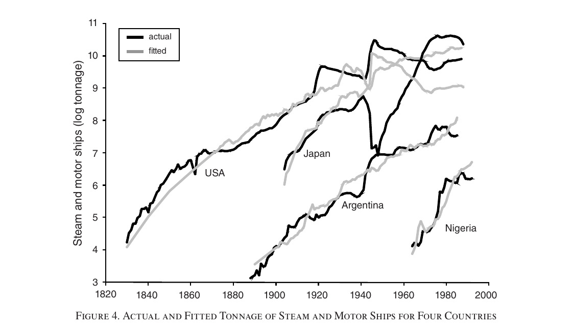
Figure 4 is the identification argument in one picture. The estimated adoption years for steam and motor ships are 1817 for the us, 1852 for Argentina, 1901 for Japan and 1957 for Nigeria. The us curve is already flattening by the mid-nineteenth century, so it is old; Argentina’s is steeper at the same dates, so it is younger; Japan’s is steeper still. Japan also sits above Argentina for most of the twentieth century, more ships at every date, and the model says that is the intensive margin, not a shorter lag. This is where the paper is most interesting. It is telling you that a country can use more of a technology than another country and still be the later adopter. It also tells you what “adoption date” means here: the us figure of 1817, against a first steamboat patent in 1788, is the date consistent with the curvature of the whole series, not the year the first steamboat sailed. (Japan’s fit has an $R^2$ of 0.04, because the model has no way to accommodate the destruction of its merchant fleet in the Second World War.)

What they find

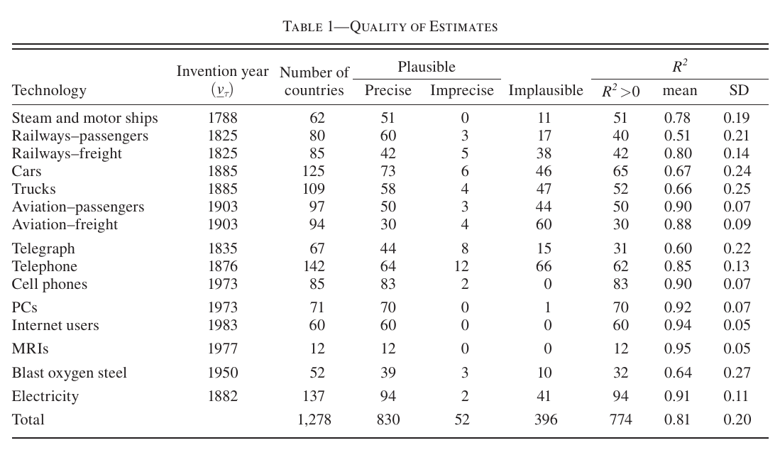
Of the 2,490 possible country–technology pairs, 1,278 have more than ten annual observations. A bit less than a third of those produce implausible estimates, adoption more than ten years before invention, and 52 more are too imprecise. The authors blame noisy series that hide the bend, convex paths in countries hit by decolonisation or civil war, and series that only begin long after adoption. Everything after that uses the 830 plausible and precise estimates, about two-thirds of the usable pairs.

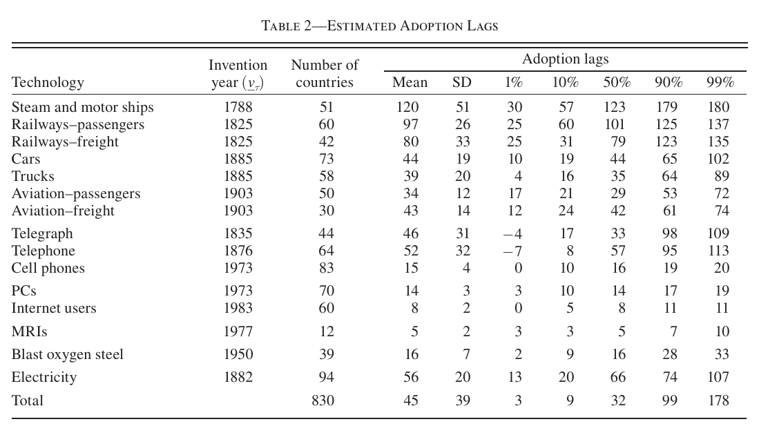
The headline in Table 2 is a mean lag of 45 years, a median of 32 and a standard deviation of 39. Steam and motor ships average 120 years and passenger railways 97, against 14 for pcs, 8 for internet users and 5 for mri scanners. It took about a century for half the countries in the sample to adopt ships and railways, and less than fifteen years for pcs and the internet.

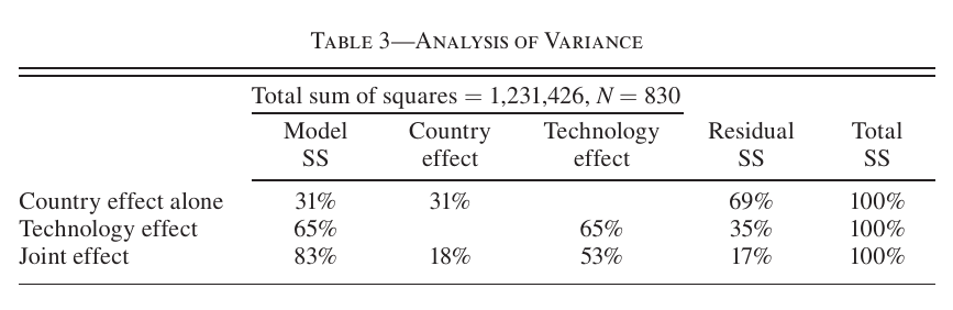
The variance decomposition in Table 3 says which technology it is matters much more than which country, by roughly two to one when each set of fixed effects is used alone. Related pairs, cars and trucks or passenger and freight aviation, get similar lag distributions without anything forcing them to.

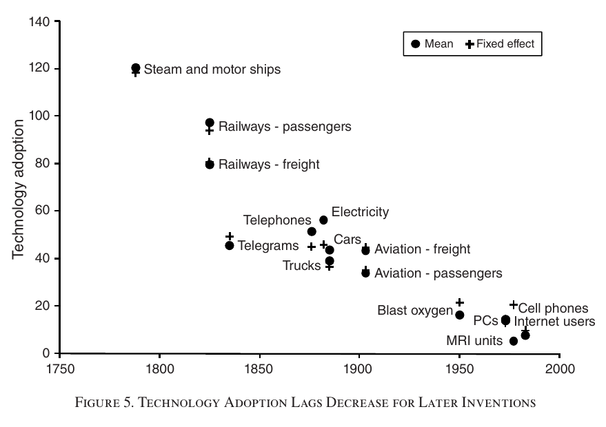
Figure 5 has the result I find most surprising. Technologies invented ten years later are adopted, on average, 4.3 years faster, and all fifteen line up on that slope. The authors say the slope before and after 1950 is almost the same, so the acceleration started long before the digital revolution or postwar globalisation, and they note that a trend like this “cannot go on forever. However, it has gone on at this pace for 200 years.” Two cautions. The before-and-after-1950 comparison is asserted in the text rather than shown, and I can’t recover it from the printed numbers: a simple regression of Table 2’s means on invention year gives about 4.9 years per decade overall, closer to 6 before 1950 and under 3 after, though five post-1950 technologies can’t settle much. And this is a pattern across invention cohorts, not evidence that a given country is getting faster at adopting a given technology.

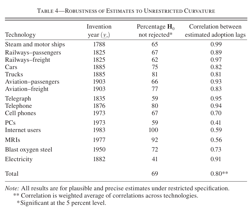
The main identifying assumption is that every country shares the us curvature $\beta_3$. The authors re-estimate without it. In Table 4, equal curvature cannot be rejected in 69% of cases, and that restricted and unrestricted lags correlate at 0.80 on a weighted average, from 0.41 for pcs to 0.99 for ships. They argue this “reduces the scope” for other sources of curvature: country-specific pro-adoption policy changes, for instance, are “very unlikely” to produce curvatures as similar as the ones observed. That is a fair point about one alternative, and I return to the others below.

The case studies are the paper’s most readable section. Japan’s lag in steam and motor ships looks Latin American, its lags for late-nineteenth-century technologies look oecd, and its lags for twentieth-century technologies look American; along the way Japanese income per head went from 42% of the oecd average in 1870 to 26% above it by 1980. The East Asian Tigers had lags for pre-1950 technologies that were often longer than sub-Saharan Africa’s, then adopted post-1950 technologies about as fast as the oecd. That lets the paper step lightly into the Young (1995) versus Hsieh (2002) argument about whether East Asian growth was accumulation or productivity. The authors’ answer is that it depends on whether capital is quality-adjusted, since a lag shortened through new embodied vintages can show up in either column. They also run a nice small test of Young (1992): if Singapore’s fast move into electronics and services kept it from learning to use older technologies efficiently, it should have shorter lags in computers and the internet than Hong Kong. It doesn’t; the two have the same lags for pcs and the internet, and Hong Kong adopted cell phones three years earlier.

From lags to income

The development-accounting step goes back to the one-sector model. If lags were the only difference between countries, then in steady state

This is eq. 32 in the paper: the left side is country $i$’s log income per head relative to the us, $\gamma = 0.014$ is postwar us tfp growth, $\alpha = 0.3$, and $D_i$ is approximated by the country fixed effect from the lag decomposition. With those numbers $\gamma/(1-\alpha) = 0.02$, so every extra year of lag costs about 2% of steady-state income per head (my arithmetic, not the paper’s), and a 50-year lag costs about one log point. Using economy-wide tfp growth assumes disembodied technologies diffuse with similar lags, and the authors say so (footnote 19).

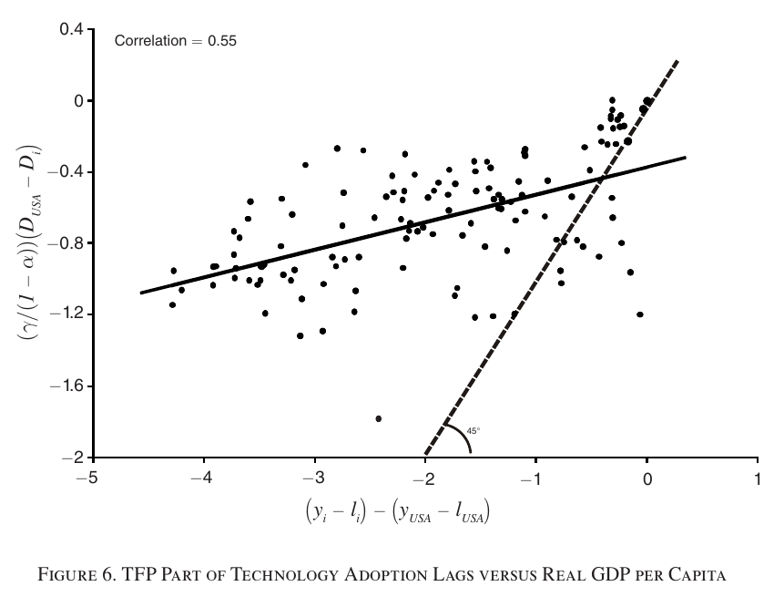
Figure 6 plots both sides for 123 countries. The correlation is 0.55, and the text says the regression slope is about 0.25, so lags explain “about one fourth” of log income differences, and the conclusion upgrades this to “at least 25 percent, if not more.” One thing doesn’t add up, though. Reading the axes, the solid line as printed runs from roughly $(-4.6, -1.1)$ to $(0.35, -0.3)$, a slope nearer 0.15 than 0.25. That might be a drafting problem with the chart rather than with the number, but 0.25 is the text’s figure, not one you can read off the exhibit. The “if not more” rests on an argument about bias: poor countries’ series for old, slow-to-diffuse technologies are often missing or implausible and drop out, which flatters their average lag and compresses the dispersion. That is plausible, but the bias goes from selection to a lower bound with an argument and no number. The fit is visibly better in the rich-country cluster at the upper right than in the long tail to the left.

For the Growth × Asset Pricing collection

The paper is about development, not asset prices, but the adoption decision in it is a valuation problem. The benefit of adopting a vintage is the market value of a firm, and the stock-market-capitalisation-to-gdp ratio $\Psi$ sits right there in eq. 15 (footnote 6: literally the market cap if every capital-good monopolist were listed). The paper uses this only on the balanced growth path, where $\Psi = \bar\Psi$ and it drops out. Taken mechanically, eq. 15 says that with barriers held fixed a valuation above its steady state would shorten the lag, so expensive equity would speed adoption. That is my reading, not the paper’s: it never discusses valuations off the balanced growth path, and in the full model $\Psi$ is itself endogenous to the lag. The part the paper does support is the timing. An invention reaches a country’s measured productivity as $e^{\gamma(t-D)}$, with a 45-year mean lag, and within a technology it arrives along a concave variety path rather than as a step. If you want a micro source for the slow, persistent growth component that long-run-risk models posit, this is a candidate, and the acceleration in Figure 5 says that delay has been shrinking for two centuries. Neither of those is a claim the paper makes or tests, and it has no returns data at all. The authors’ follow-up, Comin and Hobijn (2010), takes the same lags to postwar growth dynamics.

Weak points, my own reading (no discussant exists)

The lag is identified by one functional form. Anything else that makes a usage series concave in time, such as saturation, an S-shaped extensive margin, falling relative prices, infrastructure bottlenecks or learning, will be read as a later adoption date unless the income controls happen to soak it up. Table 4 tests whether each country’s curvature matches the us, not whether curvature comes from varieties, and a common non-variety source of concavity would pass it. The approximation behind eq. 30 is an expansion around slow embodied growth, but the term that has to be small is $\gamma_\tau(t-T)/(\mu-1)$ with $\mu - 1 = 0.3$, which is not small over a century of steamships if $\gamma_\tau$ is anything like the economy-wide 1.4% the paper calibrates (it never estimates the technology-specific $\gamma_\tau$). Footnote 17 says the estimates are robust to the approximations and shows nothing. The 830 estimates are selected partly on the outcome, since an implausible date is one the model fails to fit well, and the “at least” in “at least 25 percent” is an argument, not a bound. The cohort acceleration may be partly truncation: a technology invented in 1983 cannot yet show a 60-year lag in data ending in 2003, and countries that haven’t adopted never enter. The second step treats the us $\beta_2$ and $\beta_3$ as known, and nothing indicates that their sampling error is carried into the country lag standard errors. There are also a few typos: besides the eq. 29 sign, Table 3’s covariance share is 12% while the introduction says 11%, and the data appendix describes the telephone variable as “number of telegrams sent”, which is surely a copy-paste from the telegraph entry above it.

None of this undoes what the paper does well. It turned a pile of unlovely series on tonnage, kilowatt-hours and passenger-kilometres into adoption dates with a model behind them, and the dates mostly make sense: rich countries early, Japan catching up on schedule, the newest technologies spreading in a decade. The cost is an identifying assumption with a slightly odd implication. Under it, the best evidence that a country got a technology early is how bored its data look.

References