Geoeconomic Pressure

Christopher Clayton (Yale), Antonio Coppola (Stanford GSB), Matteo Maggiori (Stanford GSB), Jesse Schreger (Columbia). NBER Working Paper 34020, July 2025 draft, 56 printed pages; page numbers below are the paper’s printed ones. Written from the paper alone: no talk video or transcript was available, so nothing here is attributed to a presentation. One image is a slide from the authors’ own deck, used because it draws the paper’s worked example in the paper’s notation; everything else is cropped from the PDF. The authors say they intend to update the analysis frequently, so the numbers are those of this draft.

The threats you cannot see

Here is the awkward thing about studying economic coercion, and it is the same thing that makes coercion worth studying.

You are the United States. You would like ASML, a Dutch company, to stop selling advanced lithography machines to Chinese chipmakers. You have no authority over a Dutch company. The paper says a government in this position has two moves, lean on the firm directly or lean on the firm’s own government, which does have authority over it, and that “in the case of ASML the US government seems to have pursued both avenues” (p. 20). The firm-level lean was reportedly the Foreign Direct Product Rule, which “would have allowed the US government to directly regulate ASML as long as it used technology and inputs produced by US firms as part of its business” (p. 21). What passed between Washington and The Hague is, the authors note, the kind of thing that stays in confidential diplomatic channels. What came out the other end is not in doubt: “ASML faced export controls imposed by either the US or the Netherlands towards Chinese mainland producers of semiconductors such as SMIC and Yangtze Memory Technologies.”

The paper’s framework, carried over from the authors’ theory papers, has exactly two letters for this. A firm’s value is $V(x^*,Z,\theta,\tau)$, where $\theta$ is the pressure hanging over it (the threat, the thing that happens if it does not cooperate) and $\tau$ is the costly action it is being told to take (an export ban is a tax on the relevant sales with the rate set to infinity). The firm complies when $V(x^*,Z,\theta,\tau)\ge V(x^*,Z,\theta,0)$, that is, when doing as it is told beats finding out what the threat means (p. 19). The FDPR was never imposed on ASML; that is the point of a threat. The halt in China sales was, and that is the part you can see.

So the problem for anyone with a spreadsheet is that the observable ($\tau$) is the shadow of the unobservable ($\theta$), and the most successful threats are precisely the ones that never have to become policy. Drezner made the point about sanctions two decades ago and the paper cites it: if sanctions are a tool of pressure they “should frequently be threatened and rarely imposed” (p. 6). A dataset of imposed sanctions is a dataset of the threats that failed. Stack a second problem on top. Even when pressure is realized it does not come in categories. “The fundamental challenge is that pressure can take many forms,” the paper says: the instrument can be sanctions, tariffs, export controls, regulation, boycotts; the threat might or might not be carried out; the target’s response can run through supply chains, prices, quantities, investment, R&D, inventories (p. 2). And the means are usually a product, not a firm: “a firm might be a mining conglomerate, but it is only the rare earths that are being used as means of pressure” (p. 24). No codebook written in advance has the right boxes.

So ask the people it happened to

Both problems have the same shape. The information exists, in prose, in the places where someone had to explain a bad quarter. A CEO gets asked on an earnings call why China revenue fell and says something. The analyst covering the firm, who has “career incentives to accurately analyze the available information” (p. 23) and no government to placate, says it more plainly.

That is the corpus, in three pieces (Table 1, p. 8). Global earnings-call transcripts from Capital IQ via WRDS, a little over 364,000 of them for 2008 to 2025, which are the transcripts everyone uses and which are overwhelmingly American: 3,333 US firms in 2024 against 161 Chinese ones. Since China will be on one end or the other of most of the pressure, the authors add transcripts of earnings calls and investor meetings for the universe of mainland-listed A-share firms from Orbit, about 220,000 documents and 4,871 firms in 2024. And about 200,000 analyst reports from J.P. Morgan (single firms, from 2011) and Fitch’s BMI unit (country-sectors such as “Argentina Banking”, from 2017), the latter there to reach countries whose firms never hold a call and to catch what executives will not say about their own government. Roughly 785,000 documents in all.

Notice what is not in that description: nobody is required to produce any of it. The paper is explicit that “firms voluntarily choose whether to hold a call, they may have some degree of control over which questions to accept from analysts, and they choose how to answer them, all of which may be strategically motivated” (p. 48), and it lists selection into the corpus as its first limitation, with the concrete example that Russian firms largely stop appearing after 2022. The corpus is not a census. It is a very large collection of people who chose to talk.

Now the reading. The paper’s methodological claim is that this is what large language models are for: not oracles, classifiers. The old choice in text economics was between counting words, which is cheap and stupid, and hiring humans to read against a long instruction sheet, which is smart and does not scale to several hundred thousand documents. The authors run the human’s job on machines, and it is worth being precise about the machines, because “at scale” is doing real work. The baseline model is Meta’s Llama 3.3 at 70 billion parameters; Google’s Gemma 3 (27 billion) and Alibaba’s Qwen 2.5 (72 billion) are used to repeat the analysis. All inference runs locally, on Stanford’s Sherlock cluster (eight A100-80GB and four H100-80GB GPUs) and its newer Marlowe cluster, with the models quantized to four bits so that each fits on a single GPU (p. 9). The paper’s own phrase is that the approach “comes with substantial computational requirements” (p. 9). This is a research-cluster project, not a laptop project, and the two-stage design below exists, the paper says, to keep the bill down.

Stage one runs a cheap prompt over every document and returns seven yes-or-no flags, for tariffs, sanctions, export controls, boycotts, investment screening, subsidies to onshore or friendshore, and a catch-all for any geoeconomic pressure, plus a 750-word summary the authors keep for manual inspection (pp. 10–13). The definitions are conceptual, not lexical. The prompt is told to flag discussions where “the words ’tariffs,’ ‘sanctions,’ and ’export controls’ do not even appear in the text” (p. 10), and the authors name the two confusions they are trying to avoid: “a sanction imposed by the US government on firms that buy Russian oil is different from an export control on oil imposed by the Russian government on its domestic firms,” and “The word tariff is also used by utility providers and telephone companies to mean ‘fee schedule.’” The prompt’s definition of a tariff is “taxes imposed on imported foreign goods. In order to be considered tariffs, these policies must be imposed by the importing country.”

Stage two runs only on flagged documents, with a prompt specific to the instrument (in this draft, tariffs, sanctions and export controls only), and it is a questionnaire. The reproduced tariff prompt asks for a written analysis of up to 300 words, then 52 structured fields (the paper rounds this to “approximately 55”), then a 100-word summary, then a short self-evaluation of whether the structured output agrees with the written analysis (pp. 13–18). The fields are the theory’s: who is imposing, who is receiving, which products the firm sells are hit, which inputs it buys are hit, whether the tariffs are current or merely threatened, and then, for every margin from investment and labor through prices, quantities, inventories, R&D and supply-chain moves to profit margins, an up flag, a down flag and a list of countries. Every response flag carries the same instruction: set it only if the text “explicitly attributes” the change to the instrument. Free-text products get mapped to four-digit SIC codes with a sentence-embedding model and checked by hand where the match is weak; firms get their sector from Factset (p. 24).

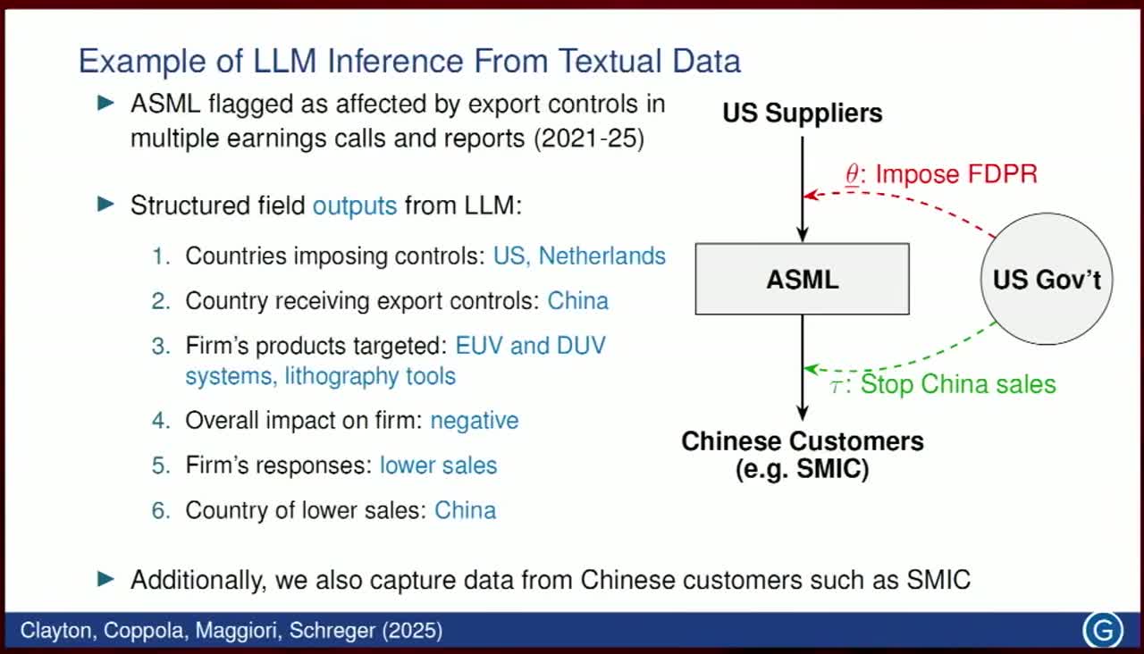
ASML is the paper’s own check that the machine reads the case the way a person would. It is flagged for export controls in 25 earnings calls between January 2021 and January 2025; the model names the imposer as the United States or the Netherlands, the receiver as China, the products as “EUV systems”, “lithography tools” and “EUV and DUV systems”, the response as lower sales in China, and the overall effect as negative (p. 21). SMIC, at the other end, is classified as negatively affected, with domestic sales down and, in its February 2022 call, domestic investment and R&D up. One episode, read from three seats.

What comes out

The aggregate series behave, which is the minimum bar.

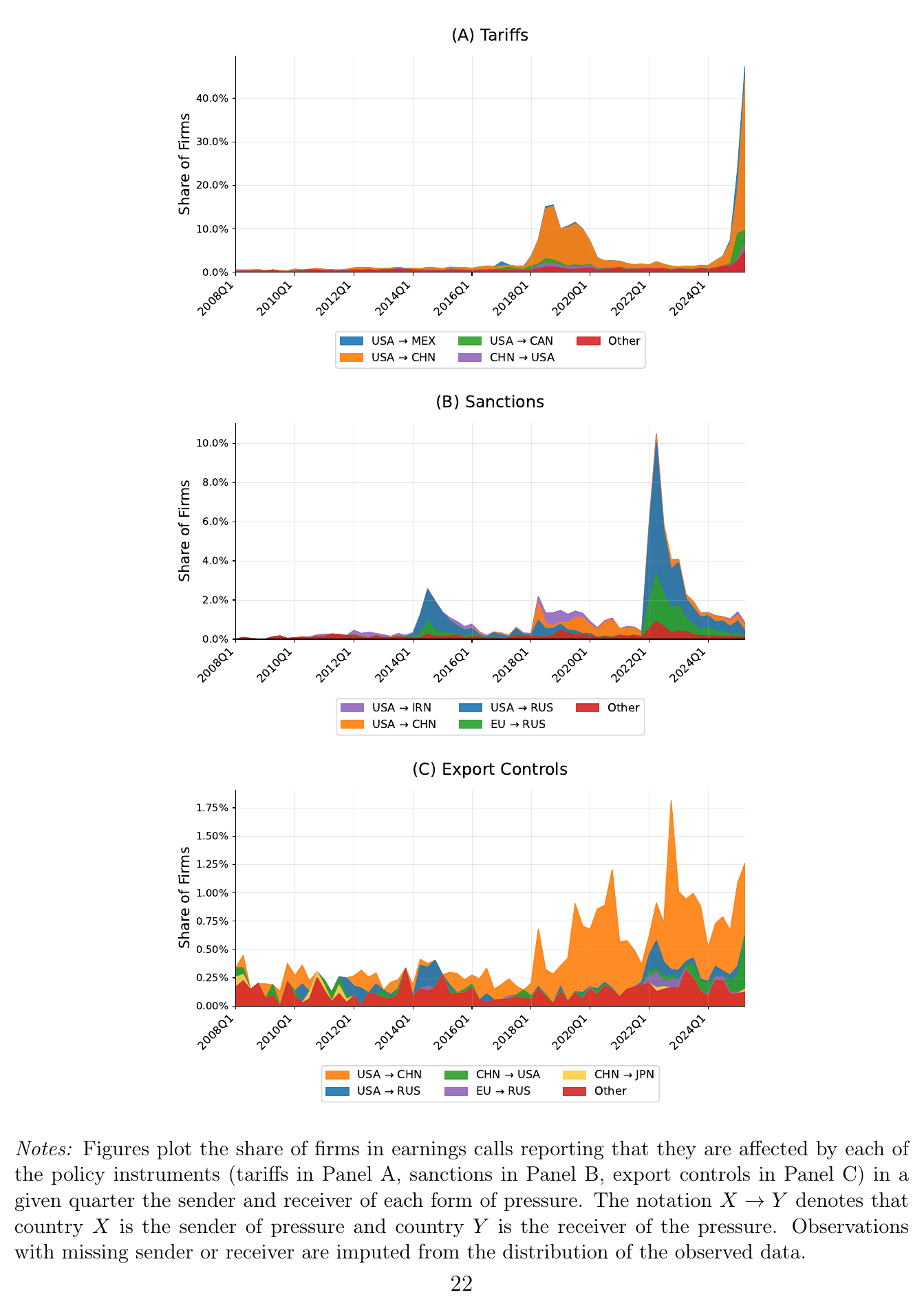
Tariff talk peaks at about 15 percent of firms in 2018–19 and passes 40 percent in the first half of 2025, both spikes driven by US tariffs on China. Sanctions spike in 2014 and 2022 with Russia’s two invasions, and the hump in between is two things: US sanctions on Iran from the second quarter of 2018, after the JCPOA withdrawal, and the Huawei and ZTE sanctions of 2019–21. Export controls trend up from 2018 and are almost entirely the United States on China (p. 23). Run the whole thing on analyst reports instead of earnings calls and the same shapes come back (Figure 13, p. 49), which is the paper’s answer to the worry that executives self-censor.

The interesting layer is who is pressing whom through which sector.

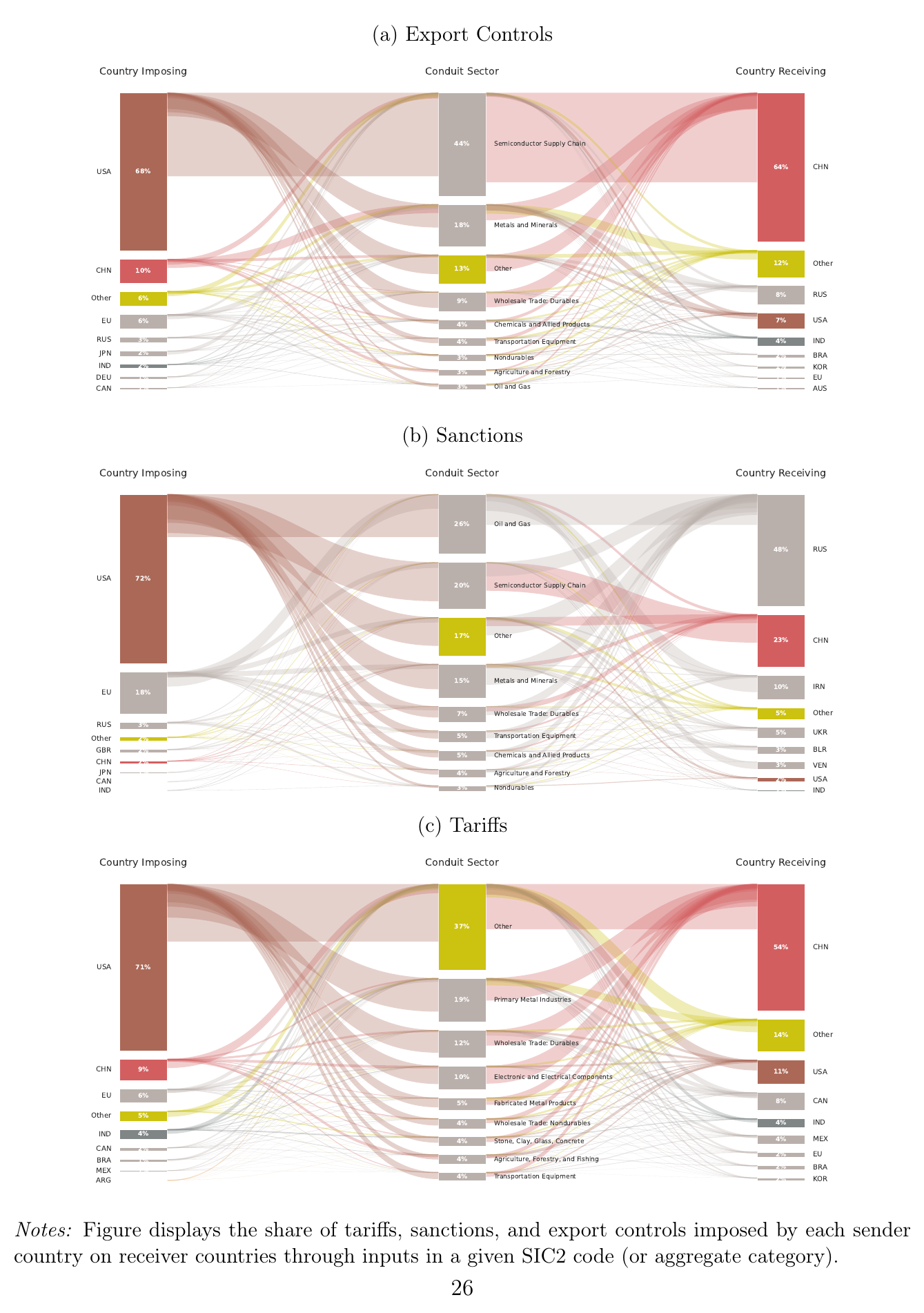
Export controls are two hegemons and a handful of sectors: the United States imposes 68 percent of them, 44 percent travel through the semiconductor supply chain, China receives 64 percent, and when China is the sender the conduit is rare earths and what is made from them, “such as magnets and batteries” (p. 25). Sanctions are wider but still legible: mostly American, mostly oil and gas, mostly Russia. Tariffs are the odd one out, and the paper’s phrasing is the one to keep. Export controls and sanctions are “small yard, high fence”; US tariffs, especially recently, are “more of a ‘whole yard, massive fence’” (p. 25).

Are the sectors the right sectors

Here the two projects meet. The authors’ coercion theory says a threat not to sell hurts the target in proportion to how much of its spending runs through the sector, how much of that sector the sender controls, and how badly the target can substitute. Take Cobb-Douglas across sectors, manufacturing only, one industry cut at a time, and the power of hegemon $m$ over target $n$ through industry $J$ is (p. 27, the display following eq. 1)

where $\Omega_{nJ}$ is the target’s expenditure share on foreign inputs in $J$, $\omega_{nJRm}$ is the share of that foreign spending the hegemon controls, $\sigma_J$ is the elasticity of substitution among foreign varieties, and $\beta$ (set to 0.8) is a returns-to-scale parameter carried over from the theory paper. The power measures are the theory paper’s own estimates, dated to 2018 trade data so that they predate the controls they are meant to explain, with elasticities from Fontagné, Guimbard and Orefice. Then ask the text which sectors the United States actually used, and run (eq. 2)

a logit of whether American firm $i$ in industry $J$ reports export controls in quarter $t$ on its industry’s power measure, reported as the average marginal semi-elasticity $\hat\delta$.

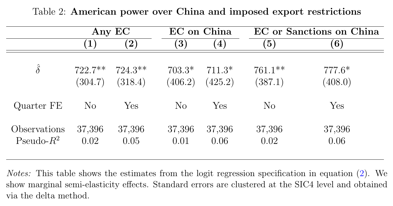
The estimate is positive in all six columns, 722.7 to 777.6 depending on how strictly “export controls on China” is defined and whether quarter fixed effects go in, and the paper’s translation is that moving an industry from the median to the 99th percentile of the power measure “increases the probability that an American firm will be involved in export controls by 1.0228 log points” (p. 28). The chokepoint idea, in other words, is not only a talking point: the sectors that show up in earnings calls are the ones the formula says would hurt. The authors list the weaknesses themselves. Indirect linkages (Taiwan in semiconductors) are ignored, and disaggregated bilateral trade data are “notoriously noisy (and estimates of elasticities even more so)” (p. 28).

One thing the paper does not do, and a reader might expect it to: it does not run this test on tariffs. The contrast between targeted export controls and broad tariffs is entirely descriptive, from the Sankey. That is fine as far as it goes, and given a “whole yard” policy you would not expect a chokepoint regression to find much, but it means the “small yard” claim has a test behind it and the “whole yard” claim has a picture.

Firms respond by category, and the categories are the theory’s

For each firm reporting being affected, every margin is coded +1 if it only went up, −1 if it only went down, 0 if both or neither, and then averaged (p. 30).

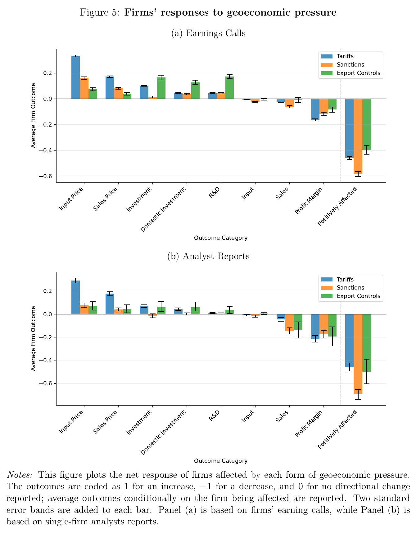
The headline split is clean. Tariffs move prices: input price up, sales price up, margin down. Export controls move R&D and investment. Sanctions mostly just hurt. But the abstract’s version undersells Figure 6, which splits the same responses by whether the firm sits in the sending country, the receiving country, or a bystander.

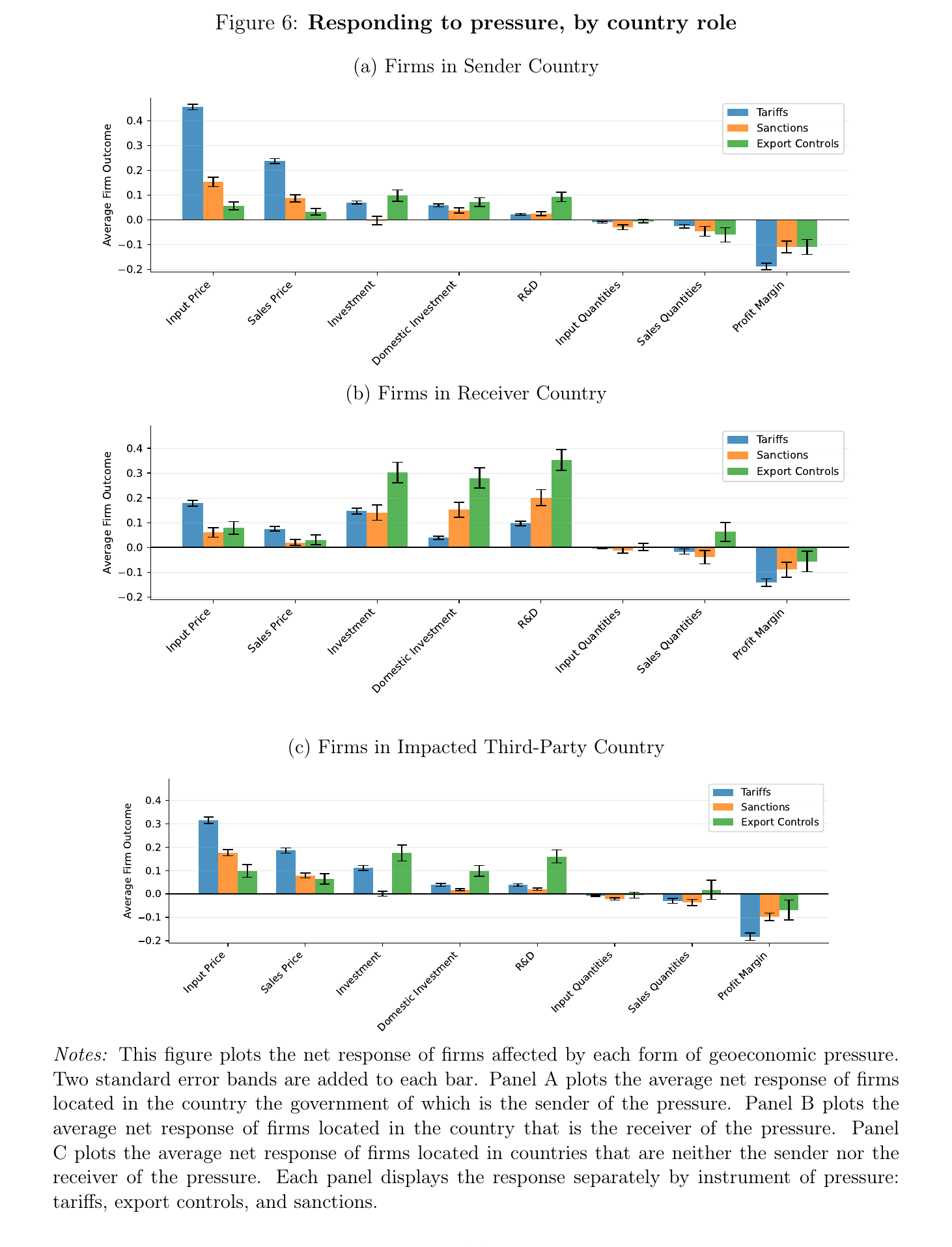
For tariffs, “nearly 50% of firms in the country imposing tariffs (‘sender’) report facing higher input prices whereas less than 20% of those in the target (‘receiver’) country do,” and the sales-price asymmetry is nearly 25 percent against under 10 (p. 34). If foreign exporters were eating the tariff you would see it on the receiver side; you do not. For export controls the sign flips: the R&D and investment “is essentially entirely concentrated in the countries targeted by the export controls” (p. 34). This is the outside option being rebuilt in real time. Rigol Technologies, a Chinese instrument maker, told a caller in September 2023 that because of the “foreign technological blockade” and export controls “there is a need to strengthen research and development, expand production,” and the model coded it as domestic investment up and R&D up (p. 34). Chinese firms also report sourcing chips from Samsung and from Vietnam and Malaysia (p. 4).

It is worth being careful about the sender side, because the tempting story is that controls induce innovation on both sides of the fence. The paper does say that “NVIDIA actively worked to develop new products to satisfy Chinese demand while remaining in legal compliance” (p. 19), and it is a good story about what a participation constraint looks like from inside a firm. But that is narrative. The classifier’s reading of NVIDIA’s November 2022 call is supply chains adjusted away from China, overall impact negative, sales roughly offset by alternative products (p. 20), and in Figure 6 the sender-side R&D response to export controls is a fraction of the receiver’s. The measured result is that targets innovate; the senders’ instruments report losing sales.

Third parties are in there too, and they are two different things: firms used as the means (a Dutch firm discussing US–China controls) and firms whose environment changed as a byproduct (an Indian company buying discounted Russian oil, p. 35). The supply-chain fields give the geography: under US tariffs, American firms report moving toward the United States, Vietnam, Malaysia and India and away from China, while Chinese firms report moving into Vietnam, Thailand, Malaysia, India and Mexico, which the paper reads as “re-routing China-US trade via East Asia and Mexico” (p. 35).

The threats, again

Back to the opening problem, because the paper answers it more directly than it advertises. Fields 2 and 3 of the tariff prompt ask separately whether the tariffs under discussion are “currently in effect” or “might be imposed in the future but are not currently in effect” (p. 14). Plot the split.

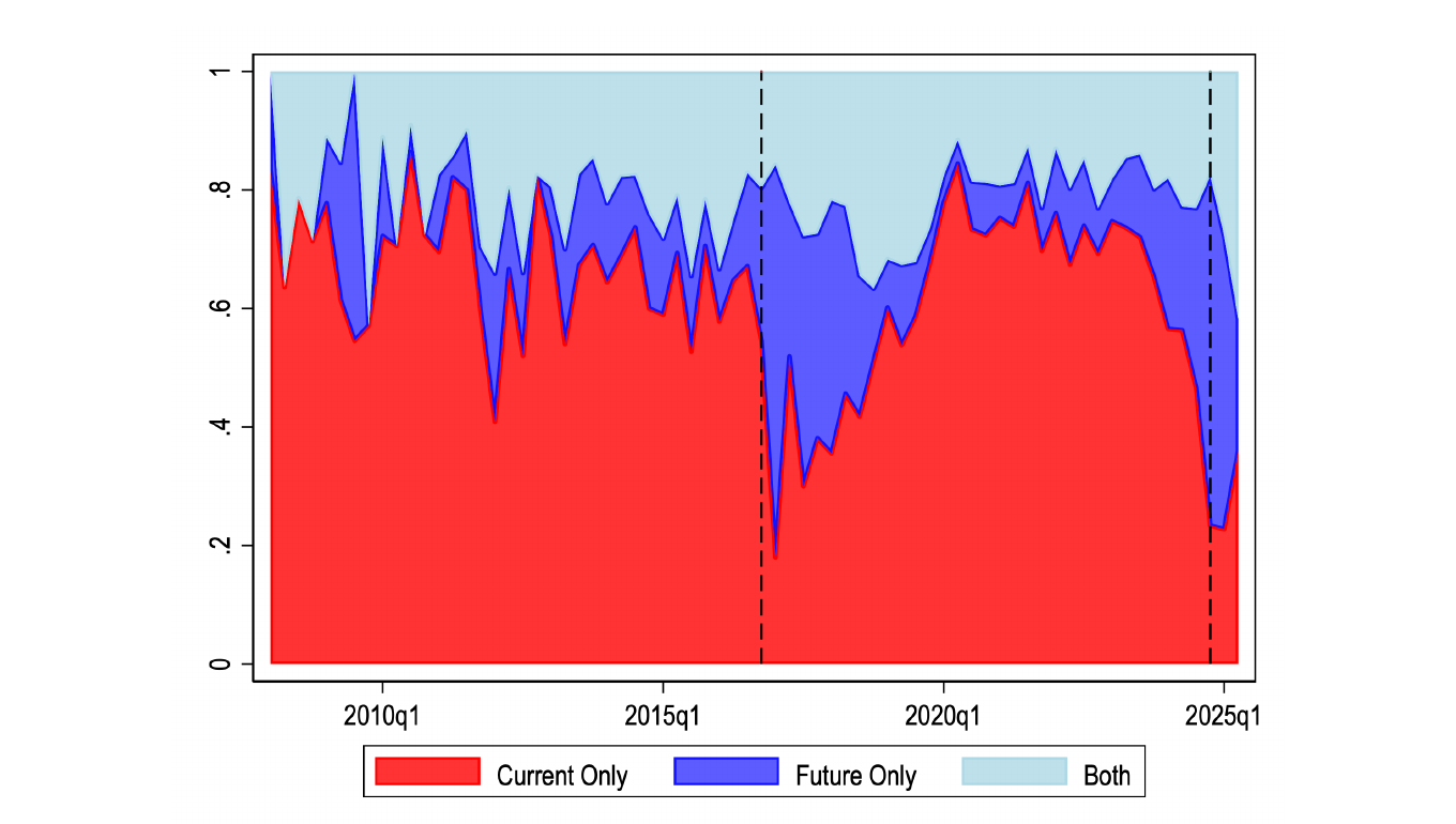
Twice, right after a November election, the share of tariff-affected firms talking only about tariffs that exist collapses from around three-quarters to about a fifth. Everyone else is reacting to tariffs that had not been imposed. In the first episode the firms “eventually transitioned by 2019 from expecting future tariffs to being affected by tariffs actually imposed”; in 2025 the two coexist, “consistent with the Trump administration both immediately imposing tariffs (for example on steel) and announcing further tariffs to be imposed at an uncertain future date” (p. 39). This is $\theta$ on a chart. The thing that leaves no trace in a tariff schedule leaves a very large trace in what firms say, which is the whole bet of the paper, and Figure 9 is the quietest exhibit in it.

Watching a tariff split into its parts

In 2025 “over 60 percent of all firms report being affected by the tariffs” (p. 4), and the share of American firms reporting being hurt “is at a high for our sample at the beginning of the second quarter of 2025” (p. 39). A tariff, as every trade student recites, is two policies in one hat, a tax on consumers of the imported good and a subsidy to its domestic producers, with a possible third leg if foreigners cut their prices to keep the market. Usually you argue about the split. Here you can watch it, because firms sort themselves.

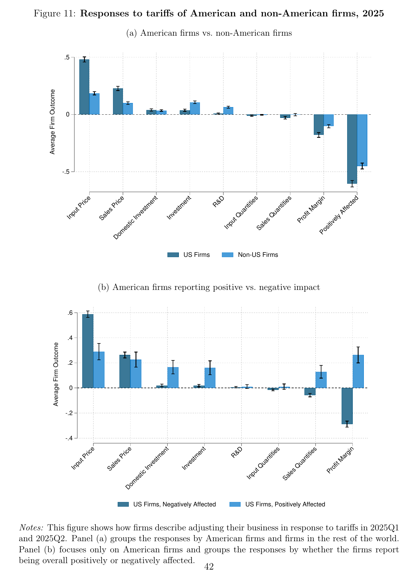
Leg one, the consumer tax: American firms are far more likely than foreign ones to report higher input prices, which the paper reads as “foreign exporters not (fully) absorbing the tariff by cutting their export prices to the US,” and more likely to report raising their own prices (p. 41). Leg two, the producer subsidy: a distinct population of American firms reports being helped, and they look different. They still report higher input prices, just far less often than the hurt firms (0.29 against 0.59; the “domestic production line” is relative, not absolute). They raise sales prices at about the same rate as the hurt firms, which for them “represents a rise in profit margins” rather than cost recovery (p. 43). Their margins go up, their quantities go up, and they are the only group reporting meaningfully higher investment and domestic investment. The paper’s example is Cleveland-Cliffs, whose executives on February 25, 2025 thanked the administration for its “courage” on steel tariffs and said “let’s produce everything here in the United States,” and which in March 2025 “laid off 1,200 workers in their Michigan and Minnesota operations, but the management maintained an upbeat assessment for the long-run impact of the tariffs” (p. 41). Leg three, the terms-of-trade gain the policy was sold on, does not appear: “we do not find systematic evidence that these entities are (planning) to cut prices at which they sell to their products to the US” (p. 4).

How much of this do you believe

The last section is the one a graduate student should read twice, and it is more careful than the version of it that tends to get repeated.

Write each measured field as $Y_{id}(\tilde p_k, m)=\bar\eta_d+\eta_{id}+\varepsilon_{idkm}$, a document’s true signal plus noise from the choice of prompt $\tilde p_k$ and model $m$. The reliability ratio $R_d=\sigma^2_{\eta,d}/(\sigma^2_{\eta,d}+\sigma^2_{\varepsilon,d})$ is the share of variance that is signal (p. 44). To estimate the noise they write 20 perturbations of every prompt (10 minor, 5 medium, 5 major, the last “meant to give as little instruction and structure to the LLM as possible”, an attempt to “deliberately ‘break’ the model”), run each under two models (Llama 3.3-70B and Gemma 3-27B; Qwen is “in ongoing work” for this part), and compute within-document variance across the 40 combinations on a stratified sample of 3,000 documents (pp. 44–45).

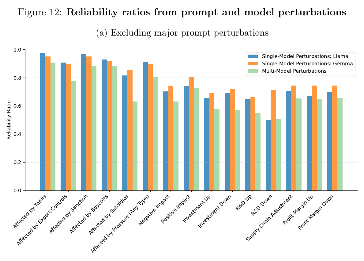
The numbers: average reliability of 78.4 percent when the model is held fixed and the prompts vary, 69.6 percent when the model varies too; including the deliberately broken prompts moves those only to 73.7 and 67.3. The interquartile range is 70.6 to 90.6 percent single-model and 62.8 to 79.4 multi-model. The stage-one flags are “often in excess of 90%”; the worst field is R&D down, but “none go below about 50%” (p. 47). Two things follow. Disagreement between models is bigger than disagreement between rewordings within a model, so anyone reporting only prompt robustness is reporting the smaller number. And the paper’s benchmark is the PSID, the CPS “or even NIPA components,” whose reliability ratios are commonly estimated in similar ranges. That is a fair benchmark and also, if you think about what people say about survey data, a modest one.

Then the paragraph that matters. Under classical measurement error the reliability ratio is exactly the attenuation you would suffer using the field as a regressor, which is why the paper says anyone doing that should use IV, and why it does not need to here: every LLM-generated field in the paper is a dependent variable (p. 47). But the perturbation analysis “is silent on whether the error is classical or not.” It can speak to variances; it “cannot make a conclusion as to whether the LLM-generated outcomes exhibit bias or correlation with other analysis variables.” Finding that out “typically requires at least a subsample that is measured without error (a ‘ground truth’ sample),” which they do not have. They point to Battaglia, Christensen, Hansen and Sacher and to Ludwig, Mullainathan and Rambachan as the econometric routes for correcting such errors, and note in a footnote that fine-tuning is being tested (p. 47). So the honest answer to “is the error classical” is: unknown, and the paper says so. There is no hand-labelled validation set and no debiasing step in this draft. A reader who wants one has to wait for it.

The paper’s list of what else can go wrong is short and worth carrying. Selection into the corpus is voluntary and strategic, and coverage collapses exactly where sanctions bite hardest. Both executives and analysts have a novelty bias: a policy gets discussed when it is new and may drop out of the text while still binding, so the “time series results should be interpreted keeping in mind this property of the data” (p. 48). And the authors take “no stance on whether the firms or the analysts are correctly assessing how policy changes will affect them nor whether they are truthfully reporting”; the model is validated only on whether it captures what the text says (p. 48). Two observations of my own. The coding is +1, −1, 0, so this measures directions, not magnitudes. And the paper itself notes that with these architectures “arbitrarily small changes to the prompt p (such as changing a single word) can in principle lead to significant changes in the output” (p. 45), which is why the perturbation set runs from cosmetic to hostile.

On reproducibility the design is straightforwardly right: open weights, local inference, zero temperature with a fixed seed to break ties, hardware held fixed, documents never leaving the servers, which is what “the same code on the same data gives the same answer” requires and what a closed model behind an API cannot promise (p. 48).

So the state of the art is a measurement instrument that reads three-quarters of a million documents on a dozen research GPUs, recovers threats that were never carried out, and carries a noise profile about the size of a good household survey. The comparison is the right one, and it has a sting in it. The survey reliability numbers it cites were learned from validation studies, matching what people told the PSID and the CPS against records of what was true. The LLM measure has the number but not, yet, the study. The paper’s own summary is that these tools “are here to stay” and “have to be handled with care, especially in terms of measurement error” (p. 5), which is what you say when you have measured the noise and not yet its shape. Everyone is going to use this anyway. The useful thing about the paper is that it went and found out how much it does not know before saying so.